Basic Variant Finding
Background
Variant calling is the process of identifying differences between two genome samples. Usually differences are limited to single nucleotide polymorphisms (SNPs) and small insertions and deletions (indels). Larger structural variation such as inversions, duplications and large deletions are not typically covered by “variant calling”.
Learning Objectives
- How to map sequence reads versus a reference
- Visualise the resultant BAM file of alignments
- Search the BAM file for variants using a SNP caller
- Filter the SNPS
Prepare reference
For variant calling, we need a reference genome that is of the same strain as the input sequence reads.
For this tutorial, our reference is the
If these files are not presently in your Galaxy history, import them from the Training dataset page.
Section 1 - Read Mapping
Map reads with BWA mem
- Go to
Tools → NGS Analysis → NGS: Mapping → Map with BWA mem - For
Will you select a reference genome from your history or use a built-in index? select Use a genome from history…. - Then for
Reference Sequence choose thewildtype.fna file. - For
Single or Paired-end reads choose Paired. - Then choose the first set of reads,
mutant_R1.fastq and second set of reads,mutant_R2.fastq . -
Leave everything else as default.
-
Click
Execute .
Convert the BAM File to a SAM file.
Now we want to look at the results. BWA mem will produce a BAM file. This is a compressed non-human readable format. So to see what it looks like, we need to convert the BAM file to a SAM file.
- Go to
Tools → NGS: Sam tools → BAM-to-SAM - Select the BAM file we just produced above and click
Execute
Now look at the contents of the resultant SAM file.
View BAM file in JBrowse
-
Go to
Statistics and Visualisation → Graph/Display Data → JBrowse -
Under
Fasta Sequence(s) choosewildtype.fna . This sequence will be the reference against which BAM file is displayed. -
For
Produce a Standalone Instance select Yes. -
For
Genetic Code choose 11: The Bacterial, Archaeal and Plant Plastid Code. -
We will now set up a new track We will choose to display the sequence reads (the .bam file)
Track 1 - sequence reads
- Click
Insert Track Group - For
Track Cateogry name it “sequence reads” - Click
Insert Annotation Track - For
Track Type choose BAM Pileups - For
BAM Track Data selectthe bam file -
For
Autogenerate SNP Track select Yes -
Click
Execute -
A new file will be created, called
JBrowse on data XX and data XX - Complete . Click on the eye icon next to the file name. The JBrowse window will appear in the centre Galaxy panel. -
On the left, tick the boxes to display the tracks
-
Use the minus button to zoom out to see:
- sequence reads and their coverage (the grey graph)
-
Use the plus button to zoom in to see:
- probable real variants (a whole column of snps)
- probable errors (single one here and there)
-
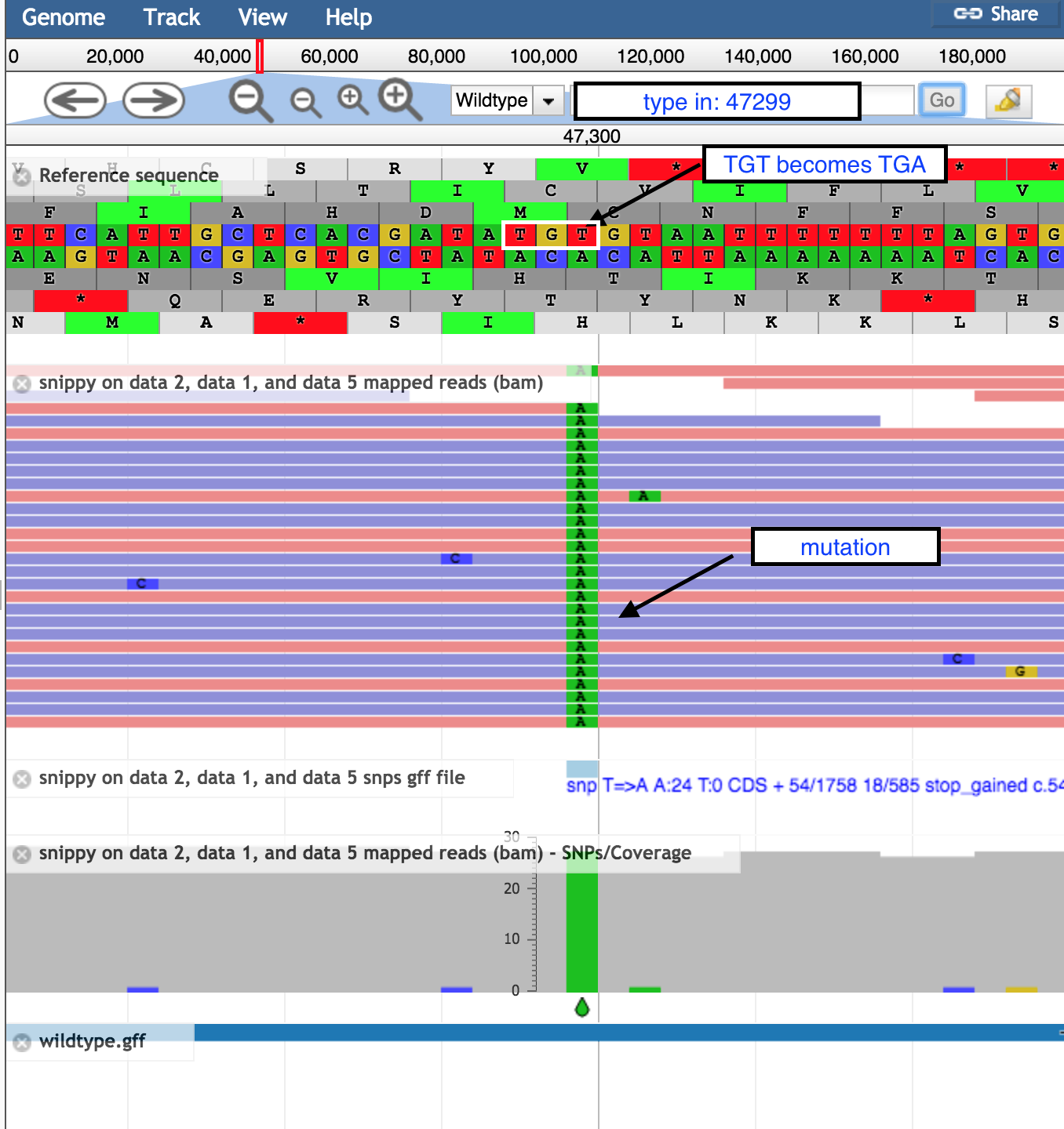
In the coordinates box, type in 47299 and then
Go to see the position of the SNP discussed above.- the correct codon at this position is TGT, coding for the amino acid Cysteine, in the middle row of the amino acid translations.
- the mutation of T → A turns this triplet into TGA, a stop codon.
End of part 1 of this exercise! More Slides!
Section 2 - Variant calling
Call variants in our BAM file with FreeBayes
- Go to
Tools &rarr NGS: Variant Analysis &rarr FreeBayes - For
Load reference genome from select History - For
BAM file select our BAM file.x: Map with BWA-MEM on data xx, data xx, and data xx (mapped reads in BAM format) - For
Use the following dataset as the reference sequence select x: Wildtype.fna - Leave everything else as default
- Click
Execute
FreeBayes will now search through each position of our BAM file and look for statistically valid variants. It uses Bayesian inference to do this. See here for details if you’re interested. (Warning! It’s complex probability theory… )
Once it’s complete you’ll see a new file in your history called x: FreeBayes on data x and data x (variants) This is a VCF file that we discussed in the slides.
Click on the “eye” icon to view the file. You’ll notice that there is a lot of header information followed by some found variants. Can you find the one we looked at earlier in our visualisation?