Trajectory analysis

Contributors

Authors: Julia Jakiela

Questions

• What is trajectory analysis?

• What are the main methods of trajectory inference?

• How are the decisions about the trajectory analysis made?

• What to take into account when choosing the method for your data?

Objectives

• Become familiar with the methods of trajectory inference

• Learn how the algorithms produce outputs

• Be able to choose the method appropriate for your specific data

• Gain insight into methods currently available in Galaxy

Requirements

• Transcriptomics
  • An introduction to scRNA-seq data analysis: slides slides

What is trajectory analysis?

.footnote[Deconinck et al. Recent advances in trajectory inference from single-cell omics data]

–

Trajectory inference (TI) methods have emerged as a novel subfield within computational biology to better study the underlying dynamics of a biological process of interest, such as:

cellular development	differentiation	immune responses
.image-40[ 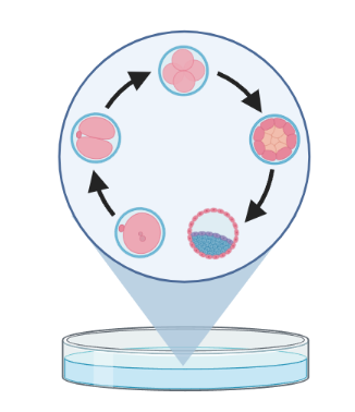]	.image-40[ 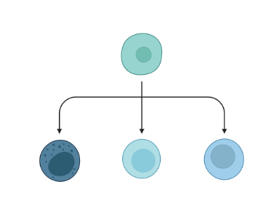]	.image-40[ ]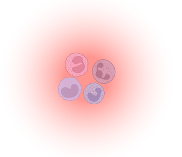

– TI allows studying how cells evolve from one cell state to another, and subsequently when and how cell fate decisions are made.

.image-40[ ]

Speaker Notes

• TI helps to understand - ‘visualise’ - the biological process that the green cell went into

Clustering, trajectory and pseudotime

.footnote[Deconinck et al. Recent advances in trajectory inference from single-cell omics data] –

.pull-left[ Clustering calculates cell similarities to identify group cell types, that can be identified based on the marker genes expressed in each cluster.

.image-75[ ]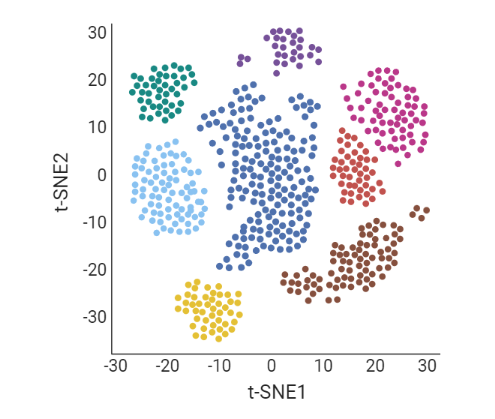

]

Speaker Notes

• axes labels - here t-SNE - the method of dimentionality reduction that was used
• each coloured group of cells => different clusters

• combine clusters and you get partition(s)

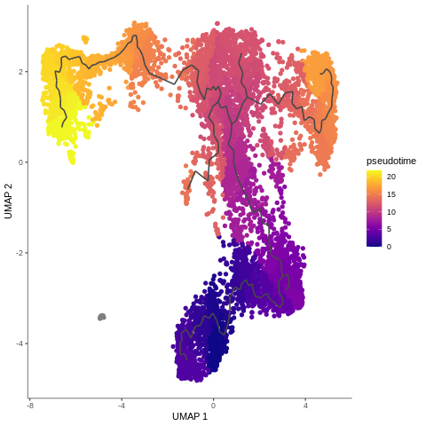
  .pull-right[ Trajectory inference helps to understand how those cell types are related - whether cells differentiate, change in response to stimuli or over time. To infer trajectories, we need data from cells at different points along a path of differentiation. This inferred temporal dimension is known as pseudotime.
  Pseudotime measures the cells’ progress through the transition.

.image-60[ ]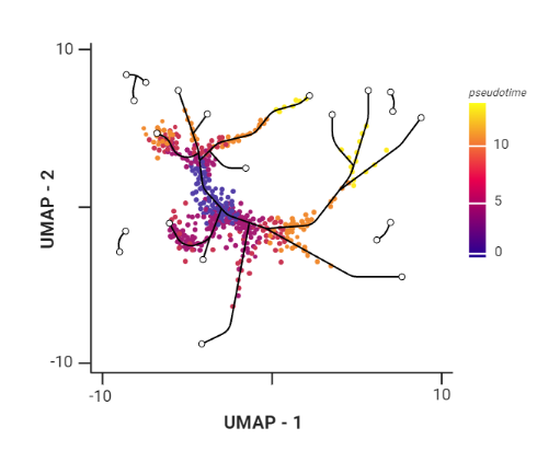

]

Speaker Notes _______________

• axes labels - here UMAP was used as the method of dimentionality reduction
• plot: usually pseudotime goes through range of colours to depict progress through the transition: here dark blue = root cells, yellow = end cells
• plot: also here’s the example of disjoint trajectories - you might choose if you want to learn single tree structure for all the partitions or learn the disjoint trajectory within each partition

Assumptions

Speaker Notes

• snapshot data with cells in different stages of differentiaiton

• multiple methods and how they work in biological context

• It would be quite difficult to analyse a sample every few seconds to see how the cells are changing. Therefore, we assume that snapshot data encompass all naïve, intermediate, and mature cell states with sufficient sampling coverage to allow the reconstruction of differentiation trajectories.
  Sagar and Grün, 2020

–

• As different TI methods make different assumptions about the data, a first choice to make is based on which biological process is to be expected: not all TI methods are designed to infer all kinds of biological processes.
  Deconinck et al., 2021

Why different TI methods are designed to infer different kinds of biological processes?

Speaker Notes There are multiple algorithms used to analyse scRNA-seq data to make it more readable. Note that this is a graph from 2016 - many new approaches has been developed since then, but this scheme shows how those methods are built. –

Look at the pipeline presented by Robrecht Cannoodt et al., 2016

–

.image-100[ ]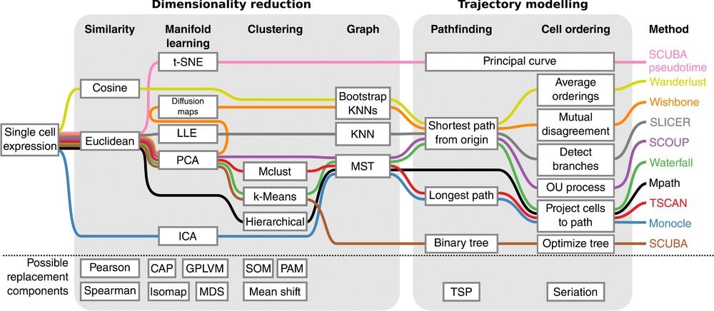

There are multiple methods using particular algorithms, or even their combinations, so you must consider which one would be best for analysing your sample.

Speaker Notes We will consider some aspects shown here to better understand similarities and differences of TI methods. Those are also the things that highly affect the output or are quite important to be aware of.

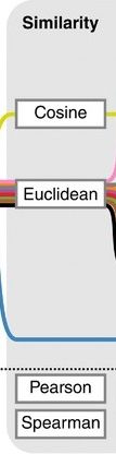
Similarity

.pull-left[

]

–

.pull-right[

• Think of similarity as a distance between cells (nearer cells - more similar)
• Euclidean distance is usually used, it’s just mathematically defined distance between two points

]

Speaker Notes

• distance matrix details: intro, slide 45

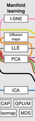
Manifold learning / dimentionality reduction

.pull-left[

]

–

.pull-right[

• Making a manifold is like making a flat map of a sphere (the Earth)
• We try to ‘flatten’ our data, changing it from high-dimensional to low-dimentional
• UMAP (Uniform Manifold Approximation and Projection) is another often used dimentionality reduction method

.image-100[ ]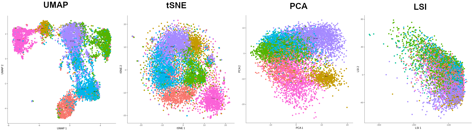

]

Speaker Notes

• Assumes that data lays on a low-dimentional manifold embedded in a higher-dimentional space
• Uses principal curves and graphs to obtain smooth trajectories
• figure shows how using different dimentionality reduction methods in Monocle3 affects the outcome

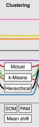
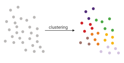
Clustering

.pull-left[

]

–

.pull-right[

• Tries to find stable cell states in the data, then connect these states to form a trajectory
• soft K-means (fuzzy clustering), Louvain, hierarchical clustering, non-negative matrix factorization

]

Speaker Notes

• cell state - which genes are expressed, which proteins are produced, what is its function, how it responds to external stimuli. Cell state changes and that’s what we want to inspect
• cell state with a particular function can be called a cell type
• methods explained in intro, slides 54 - 57
  • soft K-means: number of clusters are defined before hand, and initialised in random positions
  • Louvain: extracts communities from large networks
  • non-negative matrix factorization: splits your data up into a set of individual signals and weights to apply to those signals to recreate your original data
  • hierarchical clustering: builds a hierarchy of clusters

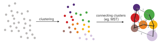
Graph-based approach

.pull-left[

]

–

.pull-right[

• think of ‘graph structure’ as the nodes (clusters with cell states) and edges (similarity, based on eg. Euclidean distance)
• Many graph-based methods start by building a **k-nearest neighbors (kNN) ** graph using the Euclidean distance
• Minimum weight spanning tree (MST) is often used to connect the clusters to each other

]

Speaker Notes

• General idea is to construct a graph representation of the cells and perform graph decomposition to reveal connected and disconnected components, or graph diffusion or traversal methods to construct the trajectory topology
• kNN explained in intro, slide 46

• MST connects clusters without any cycles and minimises the total total edge weight (cost) to ensure that the most similar clusters are connected

Graph-based approach

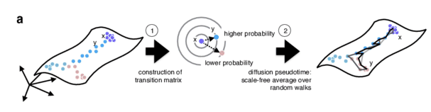
.footnote[Haghverdi et al. Diffusion pseudotime robustly reconstructs lineage branching, 2016]

.pull-left[

]

.pull-right[

• Diffusion pseudotime (DPT) uses random walks from a user-provided root cell
  • random walks between data points — path created between cells in distinct stages of the differentiation process
  • short walk => higher probability that the cells are connected
  • finding path (pseudotime) based on those probabilities

]

Extensions of trajectory inference: RNA velocity methods

.footnote[Deconinck et al. Recent advances in trajectory inference from single-cell omics data] –

• RNA velocity methods estimate the future state of a single cell captured in a static snapshot by looking at the ratios between spliced mRNA, unspliced mRNA, and mRNA degradation.
  • assuming that the cells with the highest unspliced : spliced reads are in the steady state
  • high amount of unspliced reads and low amount of spliced reads => gene is likely being turned on => higher positive velocity

.image-40[ ]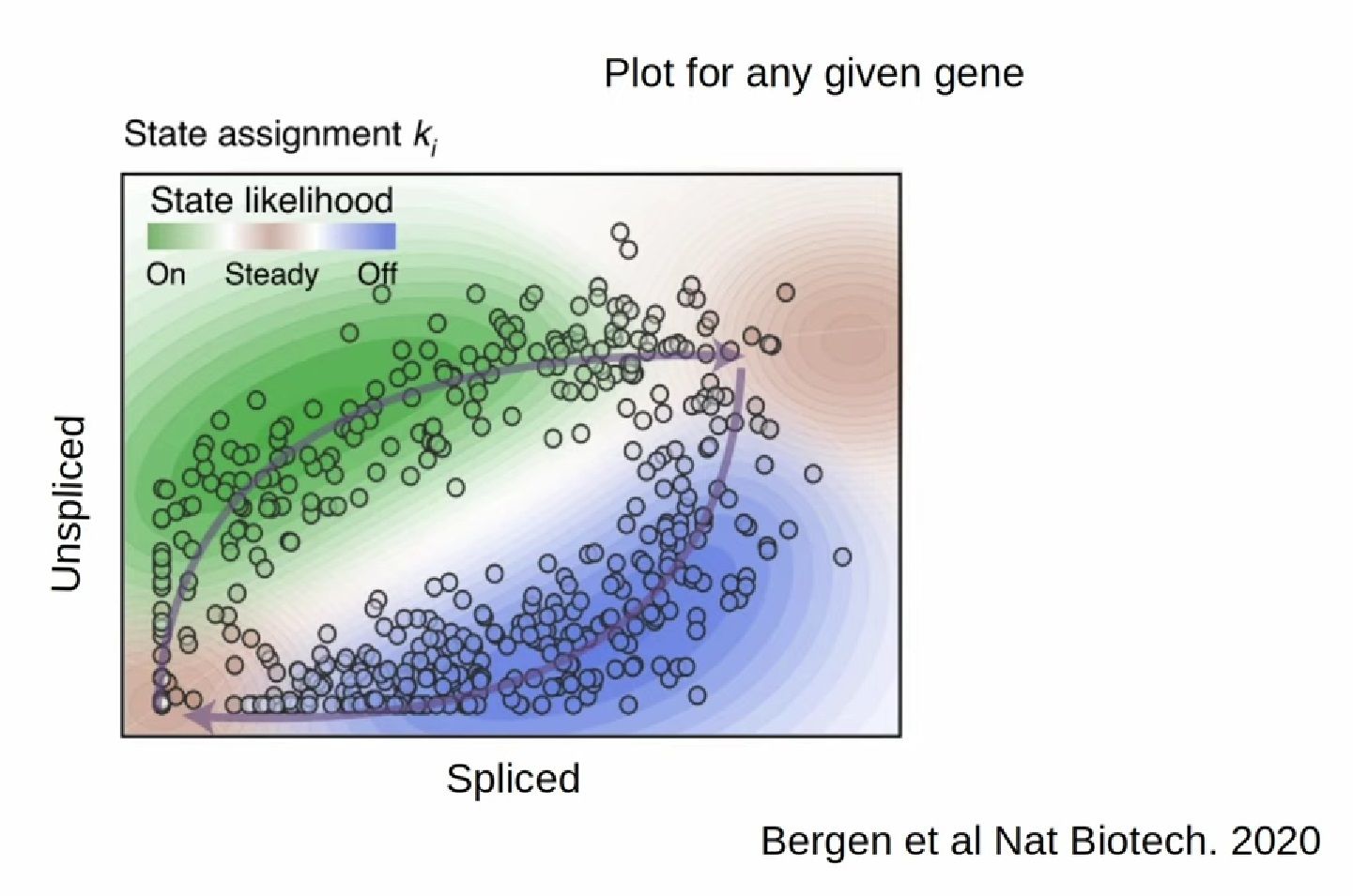

Extensions of trajectory inference: RNA velocity methods

.footnote[Deconinck et al. Recent advances in trajectory inference from single-cell omics data]

• scVelo and CellRank use this extra velocity information to construct a directed k-nearest neighbor graph, as a starting step for the TI method.

–

• This has the advantage that root cell specification is not necessary, and adds directional information to the trajectory.

–

.image-25[ ]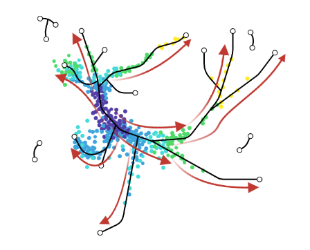

When analysing your data, consider the following:

–

.pull-left[

• Tissue from which the cells come from

• Branching points

• Supervised and unsupervised learning

• Format of the data

• Number of cells and features

• Computing power & running time

]

–

.pull-right[

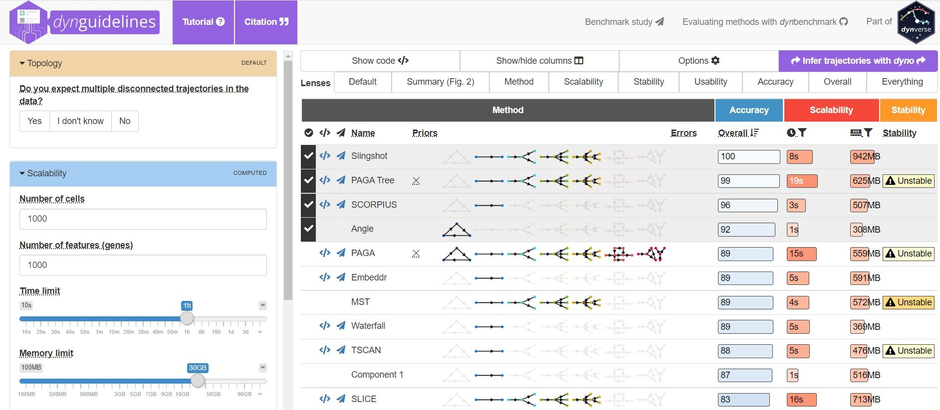
To help you evaluate which method would work best for your data, check out this awesome comparision site - dynguidelines, a part of a larger set of open packages for doing and interpreting trajectories called the dynverse.

]

When analysing your data, consider the following: Tissue from which the cells come from

–

.pull-left[

• Gives an idea of the type of cell relationships you would expect and the prior biological knowledge you can feed the method with, as well as expected cell types and potential contaminants

• You need to know about 75% of your data and verify that your analysis shows that, before you can then identify the 25% new information

• Trajectory analysis is quite a sensitive method, so always check if the obtained computational results make biological sense!

]

–

.pull-right[

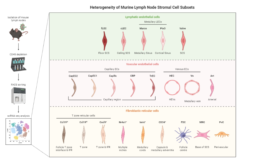
_{Reprinted from “Heterogeneity of Murine Lymph Node Stromal Cell Subsets”, by BioRender.com (2022)} ]

When analysing your data, consider the following: Branching points

–

Cells can differentiate or develop in various way, so they may exhibit different topologies.

–

![A table showing trajectory topologies: cycle, linear, bifurcation, multifurcation, tree, connected graph, disconnected graph] (../../images/scrna-casestudy-monocle/table.jpg)

When analysing your data, consider the following: Branching points

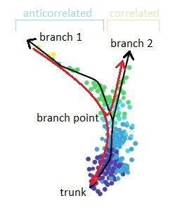
.pull-left[

• diffusion pseudotime (DPT) and branch points
• DPT does not rely on dimension reduction and can thus detect subtle changes in high-dimensional gene expression patterns

• DPT-based analysis proceeds by identifying branching points that occur after cells progress from a root cell through a common ‘trunk trajectory’
  _{L. Haghverdi et al. (2016)}

• binning and DNB (Dynamical Network Biomarker) theory
• order cells, according to the pseudotime, evenly segmented into nonoverlap bins with each bin containing X cells
• categorize DNB and non-DNB markers for each bin
• one bin contains some unassigned cells - annotated as branch bin; of the remaining bins, there are bins on the trunk, and bins for each of the branch1 and branch2
  _{Z. Chen et al. (2018)}

]

–

.pull-right[

]

Speaker Notes

• Branching points are determined by comparing two independent DPT orderings over cells, one starting at the root cell x and the other at its maximally distant cell y. The two sequences of pseudotimes are anticorrelated until the two orderings merge in a new branch, where they become correlated. This criterion robustly identifies branching points
• Branching points are identified as points where anticorrelated distances from branch ends become correlated

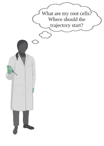
When analysing your data, consider the following: Supervised and unsupervised learning

–

.pull-left[

]

–

.pull-right[

• Some algorithms work fully unsupervised, ie. the user is not required to input any priors.

• However, many of them take the ‘starting cell’, or ‘end cell’ as information that helps to infer the trajectory which best represents the actual biological processes.

• On the other hand, priors can bias the outcome of the method, but if chosen appropriately, they are really helpful.

]

When analysing your data, consider the following: Supervised and unsupervised learning

If you know which cells are root cells, you should enter this information to the method to make the computations more precise. However, some methods use unsupervised algorithms, so you will get a trajectory based on the tools they use and topology they can infer.

–

When analysing your data, consider the following: Format of the data

–

• You have to check that your chosen method is compatible with the format of your data. If not, consider converting it or even contacting the developers to implement this into the pipeline.

–

• Other possible inputs:
• Raw (FASTQ);
• Cellxgene matrix;
• Matrix, genes & barcodes tables;
• AnnData
• RDS

–

• Powerful SCEasy tool in Galaxy to convert between formats

–

• Implementations

.image-100[ ]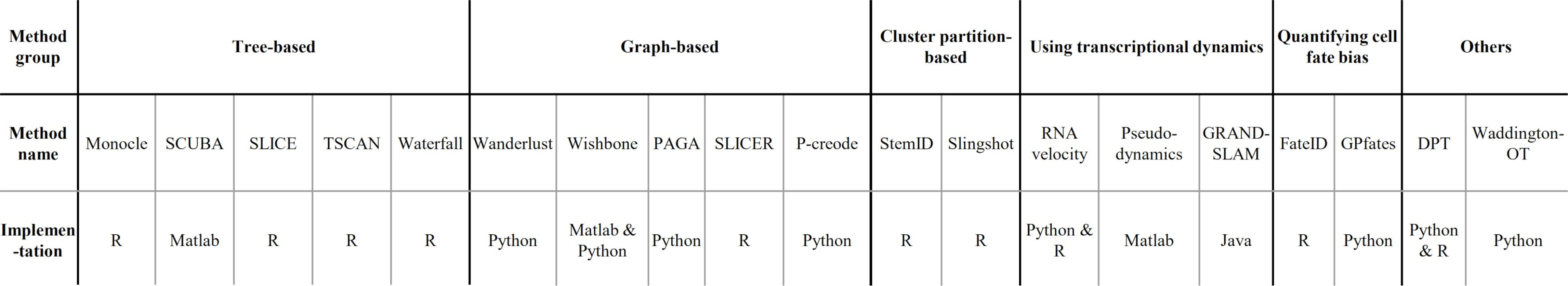

When analysing your data, consider the following: Number of cells and features

–

• The more cells and features you have, the more dimensions there are in your dataset. Therefore, it may be more computationally difficult for the particular method to reduce the dimensionality and infer the correct trajectory.

–

• For example, PAGA generally performs better than RaceID or Monocle when the dataset contains huge number of cells. (PAGA is graph-based, Monocle is tree based).

–

• Also, the more cells you have, the more insightful data you can get, but it is often associated with more noise as well. Therefore, the number of cells also impacts how you pre-process your data and how ‘pure’ it will be for trajectory analysis.

When analysing your data, consider the following: Computing power & running time

It doesn’t directly affect your analysis, however do bear in mind that calculations performed during dimensionality reduction, especially on large datasets, can be really time-consuming. Therefore, you might consider if you won’t be limited by any of those factors.

Trajectory analysis methods used in Galaxy

–

• Scanpy PAGA (Inferring Trajectories using Python (Jupyter Notebook) in Galaxy)

–

• Scanpy DPT

–

• RaceID (Downstream Single-cell RNA analysis with RaceID)

–

• Monocle3 (Trajectory Analysis using Monocle3)

–

• scVelo (coming soon)

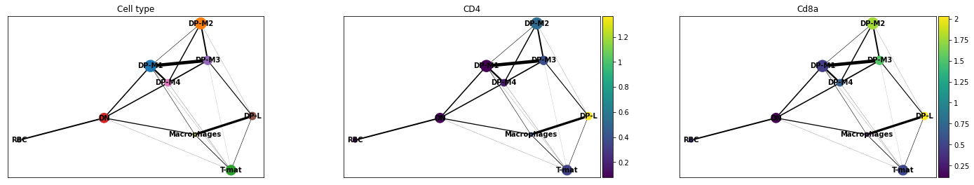
Trajectory analysis methods used in Galaxy: PAGA (Partition-based graph abstraction)

.footnote[F.A. Wolf et al. ‘PAGA: graph abstraction reconciles clustering with trajectory inference through a topology preserving map of single cells’ (2019)]

–

.pull-left[

• PAGA is used to generalise relationships between groups (clusters)
• Provides an interpretable graph-like map. The graph nodes correspond to cell groups and whose edge weights quantify the connectivity between groups
• Available within Scanpy

]

Speaker Notes

• The clustering step of RaceID identifies larger clusters of different cells by k-means clustering which is applied to the similarity matrix using the Euclidean metric

• Plot comes from Trajectory Analysis using Python (Jupyter Notebook) in Galaxy tutorial where PAGA was used from the Scanpy toolkit

–

.pull-right[

]

Speaker Notes

• But PAGA is also available as a tool in Galaxy

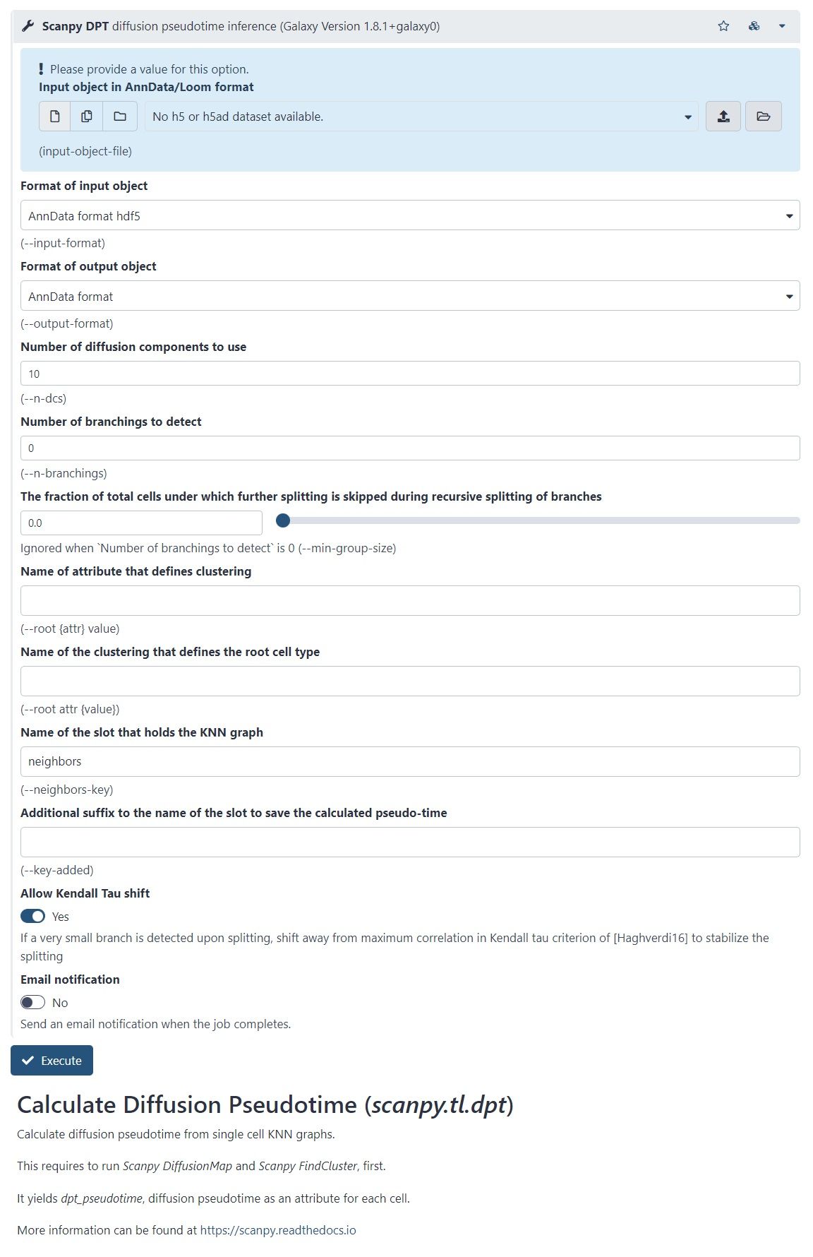
Trajectory analysis methods used in Galaxy: Diffusion Pseudotime in Scanpy

–

.pull-left[

• There is another Scanpy tool in Galaxy, which allows you to calculate diffusion pseudotime
• Based on single cell KNN graphs
• Requires to run Scanpy DiffusionMap and Scanpy FindCluster first

]

–

.pull-right[

]

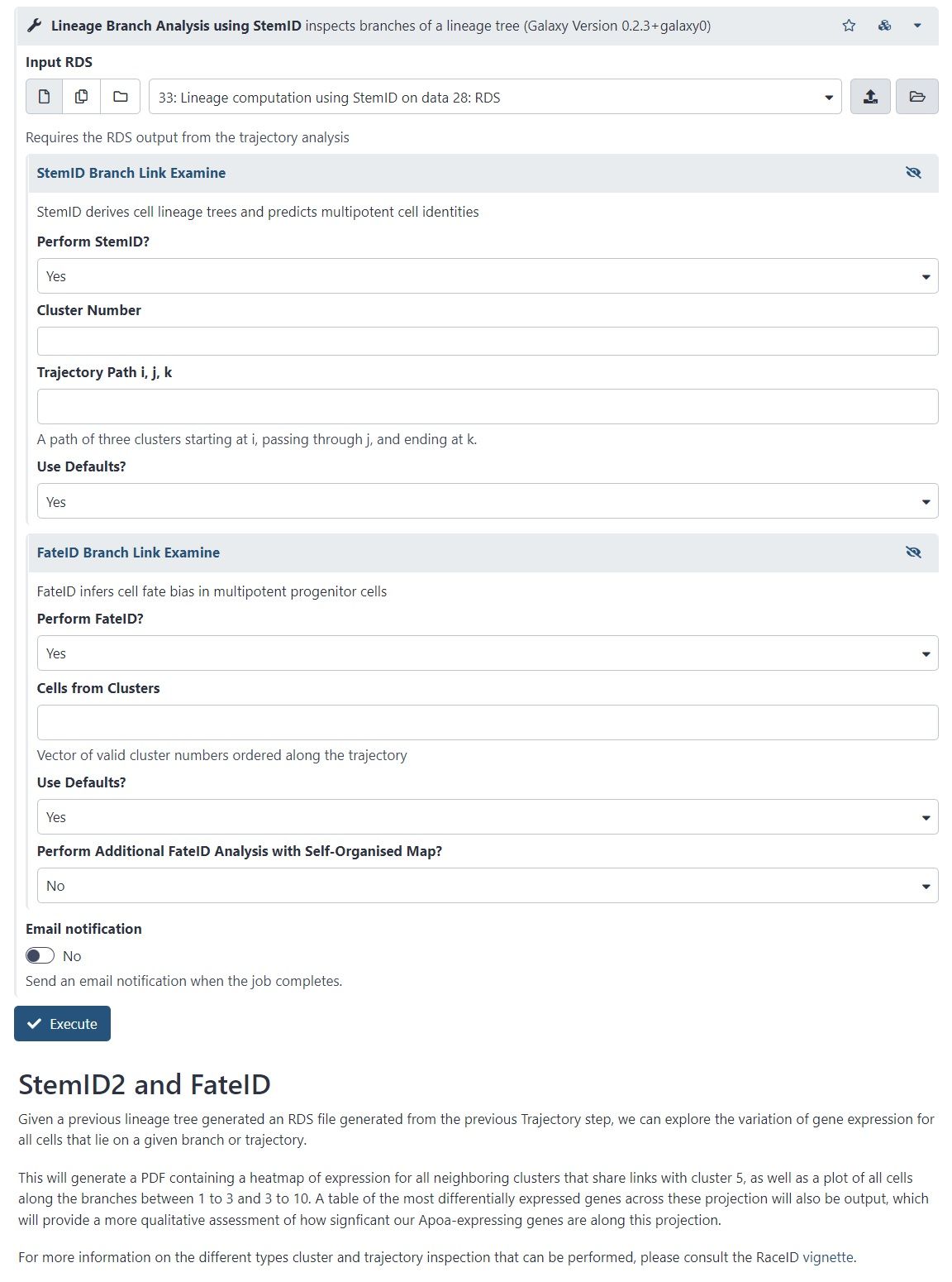
Trajectory analysis methods used in Galaxy: RaceID

.footnote[D. Grün et al., ‘Single-cell messenger RNA sequencing reveals rare intestinal cell types’ (2015)]

– .pull-left[

• StemID is a tool (part of the RaceID package) that aims to derive a hierarchy of the cell types by constructing a cell lineage tree, rooted at the cluster(s) believed to best describe multipotent progenitor stem cells, and terminating at the clusters which describe more mature cell types.
• FateID tries to quantify the cell fate bias a progenitor type might exhibit to indicate which lineage path it will pursue.
• Where StemID utilises a bottom-up approach by starting from mature cell types and working up to the multi-potent progenitor, FateID uses top-down approach that starts from the progenitor and works its way down.

]

–

.pull-right[

]

Speaker Notes

• Specific Trajectory Lineage Analysis (StemID) and Specific Trajectory Fate Analysis (FateID) in Galaxy
• Nicely described in Downstream Single-cell RNA analysis with RaceID tutorial

Trajectory analysis methods used in Galaxy: RaceID

.footnote[D. Grün et al., ‘Single-cell messenger RNA sequencing reveals rare intestinal cell types’ (2015)]

.pull-left[

• StemID is a tool (part of the RaceID package) that aims to derive a hierarchy of the cell types by constructing a cell lineage tree, rooted at the cluster(s) believed to best describe multipotent progenitor stem cells, and terminating at the clusters which describe more mature cell types.
• FateID tries to quantify the cell fate bias a progenitor type might exhibit to indicate which lineage path it will pursue.
• Where StemID utilises a bottom-up approach by starting from mature cell types and working up to the multi-potent progenitor, FateID uses top-down approach that starts from the progenitor and works its way down.

]

.pull-right[

]

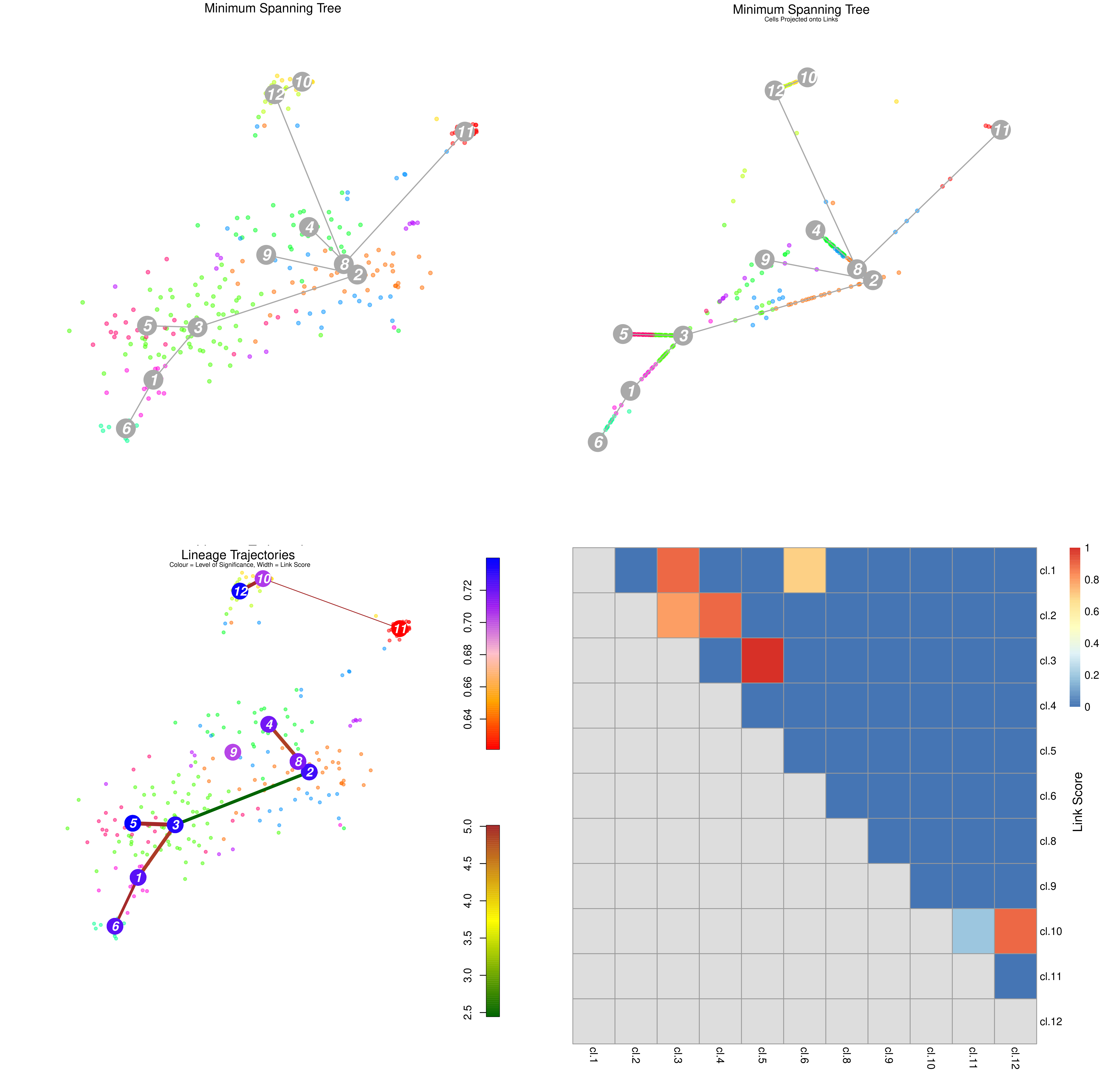
Speaker Notes From the mentioned tutorial:

• StemID Lineage Tree and Branches of significance.
  • (Top-Left) Minimum spanning tree showing most likely connections between clusters
  • (Top-Right) Minimum spanning tree with projected time series
  • (Bottom-Left) Significance between clusters
  • (Bottom-Right) Link scores between cluster-cluster pairs

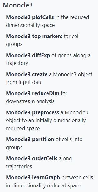
Trajectory analysis methods used in Galaxy: Monocle3

.footnote[C. Trapnell lab website, with detailed Monocle3 description and publications]

– .pull-left[

• Monocle introduced the concept of pseudotime, which is a measure of how far a cell has moved through biological progress
• Monocle uses an algorithm to learn the sequence of gene expression changes each cell must go through as part of a dynamic biological process
• General workflow:
  • Pre-process the data
  • Reduce dimensionality
  • Cluster cells
  • Learn the trajectory graph
  • Order the cells in pseudotime
• All those steps (and more) can be done using Galaxy tools!

]

–

.pull-right[

]

Speaker Notes

• Orders cells by learning an explicit principal graph from the single cell transcriptomics data with advanced machine learning techniques (Reversed Graph Embedding), which robustly and accurately resolves complicated biological processes
• Performs clustering (i.e. using t-SNE and density peaks clustering), differential gene expression testing, identifies key marker genes to discover and characterise cell types, infers trajectories
• The use of those tools was shown in (Trajectory Analysis using Monocle3 tutorial)

Trajectory analysis methods used in Galaxy: Monocle3

.footnote[C. Trapnell lab website, with detailed Monocle3 description and publications]

.pull-left[

• Monocle introduced the concept of pseudotime, which is a measure of how far a cell has moved through biological progress
• Monocle uses an algorithm to learn the sequence of gene expression changes each cell must go through as part of a dynamic biological process
• General workflow:
  • Pre-process the data
  • Reduce dimensionality
  • Cluster cells
  • Learn the trajectory graph
  • Order the cells in pseudotime
• All those steps (and more) can be done using Galaxy tools!

]

.pull-right[

]

Speaker Notes

• Example of T-cells development in pseudotime, from the mentioned Monocle3 tutorial

Trajectory analysis methods used in Galaxy: scVelo

.footnote[ Bergen et al., ‘Generalizing RNA velocity to transient cell states through dynamical modeling’ (2020)]

–

• scVelo infers gene-specific rates of transcription, splicing and degradation, and recovers the latent time of the underlying cellular processes
• think of velocities as the deviation of the observed ratio of spliced and unspliced mRNA from an inferred steady state
• Compatible with scanpy and hosts efficient implementations of all RNA velocity models
  The originally proposed framework obtains velocities as the deviation of the observed ratio of spliced and unspliced mRNA from an inferred steady state

.image-25[ ]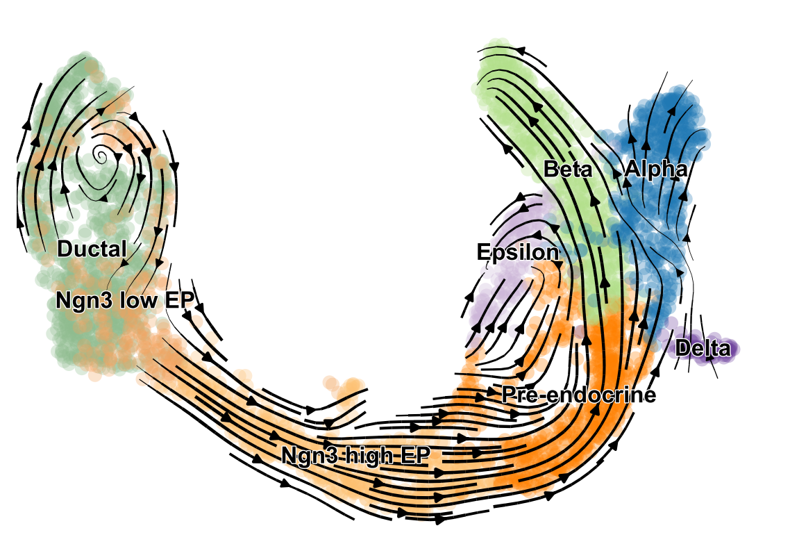

Key Points

• Trajectory analysis in pseudotime is a powerful way to get insight into the differentiation and development of cells.
• There are multiple methods and algorithms used in trajectory analysis and depending on the dataset, some might work better than others.
• Trajectory analysis is quite sensitive and thus you should always check if the output makes biological sense.

Thank you!