Cheminformatics is the use of computational techniques and information about molecules to solve problems in chemistry. This involves a number of steps: retrieving data on chemical compounds, sorting data for properties which are of interest, and extracting new information. This tutorial will provide a brief overview of all of these, centered around protein-ligand docking, a molecular modelling technique. The purpose of protein-ligand docking is to find the optimal binding between a small molecule (ligand) and a protein. It is generally applied to the drug discovery and development process with the aim of finding a potential drug candidate. First, a target protein is identified. This protein is usually linked to a disease and is known to bind small molecules. Second, a ‘library’ of possible ligands is assembled. Ligands are small molecules that bind to a protein and may interfere with protein function. Each of the compounds in the library is then ‘docked’ into the protein to find the optimal binding position and energy.
Docking is a form of molecular modelling, but several simplifications are made in comparison to methods such as molecular dynamics. Most significantly, the receptor is generally considered to be rigid, with covalent bond lengths and angles held constant. Charges and protonation states are also not permitted to change. While these approximations reduce accuracy to some extent, they increase computational speed, which is necessary to screen a large compound library in a realistic amount of time.
In this tutorial, you will perform docking of ligands into the N-terminus of Hsp90 (heat shock protein 90). The tools used for docking are based on the open-source software AutoDock Vina (Trott and Olson 2009).
The 90 kDa heat shock protein (Hsp90) is a chaperone protein responsible for catalyzing the conversion of a wide variety of proteins to a functional form; examples of the Hsp90 clientele, which totals several hundred proteins, include nuclear steroid hormone receptors and protein kinases. The mechanism by which Hsp90 acts varies between clients, as does the client binding site; the process is dependent on post-translational modifications of Hsp90 and the identity of co-chaperones which bind and regulate the conformational cycle.
Due to its vital biochemical role as a chaperone protein involved in facilitating the folding of many client proteins, Hsp90 is an attractive pharmaceutical target. In particular, as protein folding is a potential bottleneck to slow cellular reproduction and growth, blocking Hsp90 function using inhibitors which bind tightly to the ATP binding site could assist in treating cancer; for example, the antibiotic geldanamycin and its analogs are under investigation as possible anti-tumor agents.
For this exercise, we need two datasets: a protein structure and a library of compounds. We will download the former directly from the Protein Data Bank; the latter will be created by searching the ChEMBL database (Gaulton et al. 2016).
Get data
Hands-on: Data upload
Create a new history for this tutorial
Search Galaxy for the Get PDBTool: toolshed.g2.bx.psu.edu/repos/bgruening/get_pdb/get_pdb/0.1.0 tool. Request the accession code 2brc.
Rename the dataset to ‘Hsp90 structure’
Check that the datatype is correct (PDB file).
Click on the galaxy-pencilpencil icon for the dataset to edit its attributes
In the central panel, click on the galaxy-chart-select-dataDatatypes tab on the top
Select datatypes
tip: you can start typing the datatype into the field to filter the dropdown menu
Click the Save button
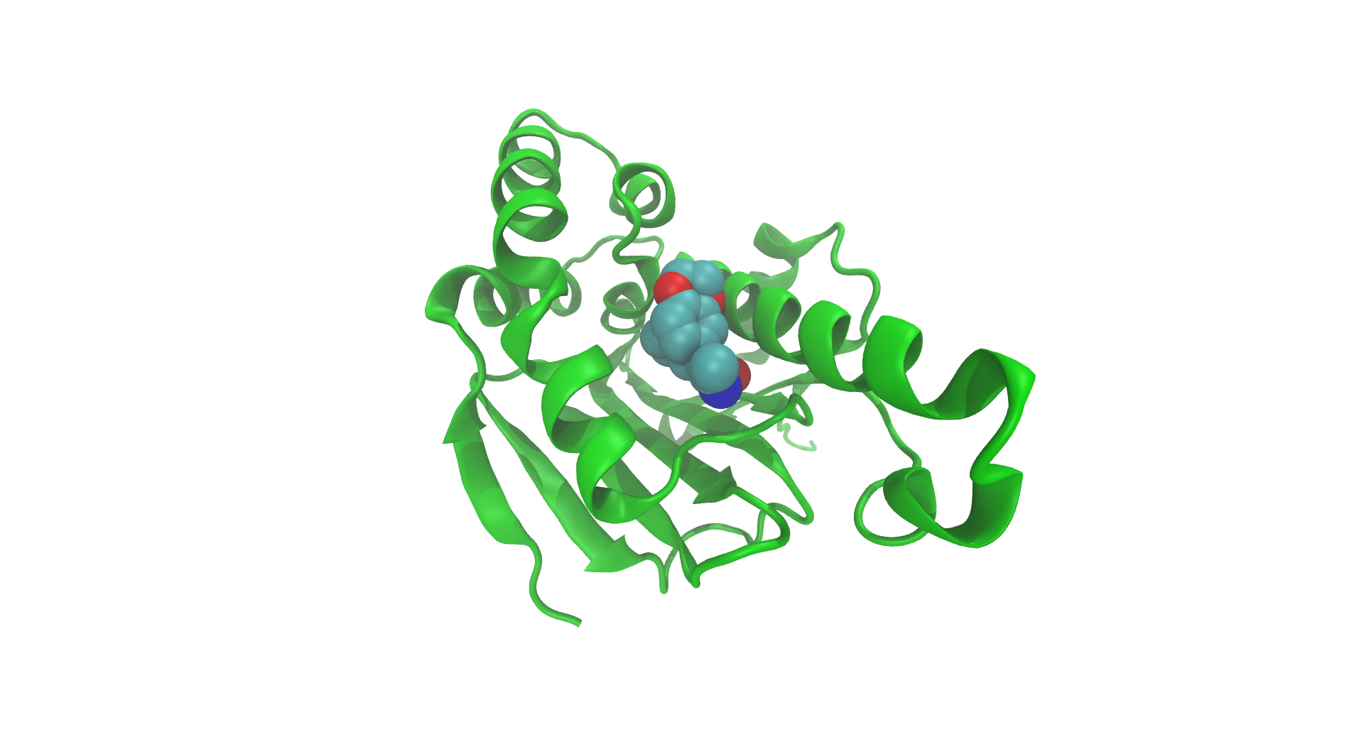
Figure 1: Structure of Hsp90 N-terminus, as recorded on the PDB. Visualization produced using VMD (Humphrey et al. 1996).
Separating protein and ligand structures
You can view the contents of the downloaded PDB file by pressing the ‘View data’ icon in the history pane. After the header section (about 500 lines), the atoms of the protein and their coordinates are listed. The lines begin with ATOM. At the end of the file, the atomic coordinates of the ligand and the solvent water molecules are also listed, labelled HETATM. We will use the grep tool to separate these molecules into separate files, and then convert the ligand file into SDF/MOL format using the ‘Compound conversion’ tool, which is based on OpenBabel, an open-source library for analyzing chemical data (O’Boyle et al. 2011).
Grep is a command-line tool for searching text files for lines which match a search query.
There is a Galaxy tool available based on grep, which we will apply to the downloaded PDB tool.
Hands-on: Separate protein and ligand
Search in textfiles (grep)Tool: toolshed.g2.bx.psu.edu/repos/bgruening/text_processing/tp_grep_tool/1.1.1 with the following parameters:
All other parameters can be left as their defaults.
Rename the dataset ‘Protein (PDB)’.
The result is a file with all non-protein (HETATM) atoms removed.
Search in textfiles (grep)Tool: toolshed.g2.bx.psu.edu/repos/bgruening/text_processing/tp_grep_tool/1.1.1 with the following parameters. Here, we use grep again to produce a file with only non-protein atoms.
param-file“Regular Expression”: CT5 (the name of the ligand in the PDB file)
All other parameters can be left as their defaults.
Rename the dataset ‘Ligand (PDB)’.
This produces a file which only contains ligand atoms.
Compound conversionTool: toolshed.g2.bx.psu.edu/repos/bgruening/openbabel_compound_convert/openbabel_compound_convert/3.1.1+galaxy0 with the following parameters:
param-file“Molecular input file”: Ligand PDB file created in step 2.
param-file“Output format”: MDL MOL format (sdf, mol)
param-file“Add hydrogens appropriate for pH”: 7.4
All other parameters can be left as their defaults.
Change the datatype to ‘mol’ and rename the dataset ‘Ligand (MOL)’.
Applying this tool will generate a representation of the structure of the ligand in MOL format.
At this stage, separate protein and ligand files have been created. Next, we want to generate a compound library we can use for docking.
Creating and processing the compound library
In this step we will create a compound library, using data from the ChEMBL database.
Multiple databases are available online which provide access to chemical information, e.g. chemical structures, reactions, or literature. In this tutorial, we use a tool which searches the ChEMBL database. There are also Galaxy tools available for downloading data from PubChem.
We will generate our compound library by searching ChEMBL for compounds which have a similar structure to the ligand in the PDB file we downloaded in the first step. There is a Galaxy tool for accessing ChEMBL which requires data input in SMILES format; thus, the first step is to convert the ‘Ligand’ PDB file to a SMILES file. Then the search is performed, returning a SMILES file. For docking, we would like to convert to SDF format, which we can do once again using the ‘Compound conversion’ tool.
Hands-on: Generate compound library
Compound conversionTool: toolshed.g2.bx.psu.edu/repos/bgruening/openbabel_compound_convert/openbabel_compound_convert/3.1.1+galaxy0 with the following parameters:
Rename the output of the ‘compound conversion’ step to ‘Ligand SMILES’.
Search ChEMBL databaseTool: toolshed.g2.bx.psu.edu/repos/bgruening/chembl/chembl/0.10.1+galaxy4 with the following parameters:
param-file“SMILES input type”: File
param-file“Input file”: ‘Ligand SMILES’ file
param-file“Search type”: Similarity
param-file“Tanimoto cutoff score”: 40
param-file“Filter for Lipinski’s Rule of Five”: Yes
All other parameters can be left as their defaults.
Question
Why are compounds filtered for Lipinski’s Rule of Five?
Lipinski’s rule of five is an empirical rule which can be used to determine the ‘druglikeness’ of a molecule. The rule consists of four criteria which relate to the pharmacokinetics of the molecule. The rule is discussed in (Lipinski 2004), or you can also read more on Wikipedia.
Optional: experiment with different combinations of options - adding different filters, adjusting the Tanimoto coefficient.
Check that the datatype is correct (smi). This step is essential, as Galaxy does not automatically detect the datatype for SMILES files.
Click on the galaxy-pencilpencil icon for the dataset to edit its attributes
In the central panel, click on the galaxy-chart-select-dataDatatypes tab on the top
Select datatypes
tip: you can start typing the datatype into the field to filter the dropdown menu
Click the Save button
Rename dataset ‘Compound library’.
A number of users encounter issues with the ChEMBL tool - sometimes the tool fails, or the output is returned successfully but is empty. If this happens to you, try the following:
Rerun the tool - if a transient error on the ChEMBL server was at fault, this might be enough to fix it.
Try modifying some of the parameters. For example, reducing the Tanimoto coefficient should increase the number of compounds returned.
If all else fails, you can use the following list of SMILES:
Don’t worry if you can’t get it to work - successfully generating this list is a very minor part of the tutorial!
There are some other tools available, which will not be used in this tutorial, which help to develop a more focused compound library. For example, the ‘Natural product likeness calculator’ and ‘Drug-likeness’ tools assign a score to compounds based on how similar they are to typical natural products and drugs respectively, which could then be used to filter the library. If you are interested, you can try testing them out on the library just generated.
If you try using this tutorial using your own data, you might encounter some issues. Important things to remember:
If you encounter an error, check the SMILES file only has a single column. Additional columns can be removed using the ‘Cut’ tool.
If the output file is empty, it may be that the ChEMBL database doesn’t have any compounds similar to the input. Consider lowering the Tanimoto coefficient to 70 if this is the case and removing filters (including the Lipinski RO5 filter). If this doesn’t help, you will have to use another source of chemical data (e.g. PubChem).
Finally, please remember this step is totally optional if you already have a list of compounds for docking (in SMILES or another format). In this case you can upload them to Galaxy and continue with the next step.
SMILES and SD-files both represent chemical structures. A SMILES file represents the 2D structure of a molecule as a chemical graph. In other words, it states only the atoms and the connectivity between them. An example of a SMILES string (taken from the ligand in the PDB file) is c1c2OCCOc2ccc1c1c(C)[nH]nc1c1cc(CC)c(O)cc1O. For more information on how the notation works, please consult the OpenSMILES specification or the description provided by Wikipedia. A more comprehensive alternative to the SMILES system is the International Chemical Identifier (InChI).
Neither SMILES nor InChI format contain the three-dimensional structure of a molecule. By contrast, the SDF (structure data file) format encodes three-dimensional atomic coordinates of a structure, similar to a PDB file.
In a previous step, we also generated a MOL file - this format is closely related to the SDF format. The difference is that MOL files can store only a single molecule, whereas SD-files can encode single or multiple molecules. Multiple molecules are separated by lines containing four dollar signs ($$$$).
For docking, we need the three-dimensional coordinates of the ligand; thus, we want to convert from SMILES to SDF format.
Prepare files for docking
A processing step now needs to be applied to the protein structure and the docking candidates - each of the structures needs to be converted to PDBQT format before using the AutoDock Vina docking tool.
Further, docking requires the coordinates of a binding site to be defined. Effectively, this defines a ‘box’ in which the docking software attempts to define an optimal binding site. In this case, we already know the location of the binding site, since the downloaded PDB structure contained a bound ligand. There is a tool in Galaxy which can be used to automatically create a configuration file for docking when ligand coordinates are already known.
Hands-on: Generate PDBQT and config files for docking
Prepare receptorTool: toolshed.g2.bx.psu.edu/repos/bgruening/autodock_vina_prepare_receptor/prepare_receptor/1.5.7+galaxy0 with the following parameters:
param-file“Select a PDB file”: ‘Protein’ PDB file.
Compound conversionTool: toolshed.g2.bx.psu.edu/repos/bgruening/openbabel_compound_convert/openbabel_compound_convert/3.1.1+galaxy0 with the following parameters:
Calculate the box parameters for an AutoDock Vina jobTool: toolshed.g2.bx.psu.edu/repos/bgruening/autodock_vina_prepare_box/prepare_box/2021.03.4+galaxy0 with the following parameters:
param-file“Input ligand or pocket”: Ligand (MOL) file.
param-file“x-axis buffer”: 5
param-file“y-axis buffer”: 5
param-file“z-axis buffer”: 5
param-file“Random seed”: 1
Rename to ‘Docking config file’.
Perhaps you are interested in a system which does not have a ligand within the binding site (an apoprotein). In this case you need to run the fpocket tool to identify potential binding sites in the protein structure - take a look at the following (optional) section.
If the structure contains no ligand in complex with the protein (i.e. apoprotein), there is an additional step of identifying the binding site. Software is available for automatic detection of pockets which may be promising candidates for ligand binding sites. For example, let’s try out the fpocket tool (Le Guilloux et al. 2009) on the Hsp90 structure, imagining we don’t have access to the file containing the ligand coordinates.
Hands-on: Finding binding sites using fpocket
fpocketTool: toolshed.g2.bx.psu.edu/repos/bgruening/fpocket/fpocket/3.1.4.2+galaxy0 with the following parameters:
param-file“Input file”: Protein (PDB) file.
param-file“Type of pocket to detect”: Small molecule binding sites
param-file“Output files”: select PDB files containing the atoms in contact with each pocket, Log file containing pocket properties.
Calculate the box parameters for an AutoDock Vina jobTool: toolshed.g2.bx.psu.edu/repos/bgruening/autodock_vina_prepare_box/prepare_box/2021.03.4+galaxy0 with the following parameters:
param-file“Input ligand or pocket”: pocket2 PDB file from the Atoms in contact with each pocket collection.
param-file“x-axis buffer”: 5
param-file“y-axis buffer”: 5
param-file“z-axis buffer”: 5
param-file“Exhaustiveness (optional)”: 1
param-file“Random seed”: 1
Rename to ‘Docking config file derived from pocket’.
The fpocket tool generates two different outputs: a Pocket properties log file containing details of all the pockets which fpocket found in the protein. The second output is a collection (a list) containing one PDB file for each of the pockets. Each of the PDB files contains only the atoms in contact with that particular pocket. Note that fpocket assigns a score to each pocket, but you should not assume that the top scoring one is the only one where compounds can bind! For example, the pocket where the ligand in the 2brc PDB file binds is ranked as the second-best according to fpocket.
You can compare the config file generated with the one generated from the ligand directly - if you picked the right pocket (pocket2) the coordinates should be pretty similar.
Docking
Now that the protein and the ligand library have been correctly prepared and formatted, docking can be performed.
Hands-on: Perform docking
DockingTool: toolshed.g2.bx.psu.edu/repos/bgruening/autodock_vina/docking/1.1.2+galaxy0 with the following parameters:
param-file“Receptor”: ‘Protein PDBQT’ file.
param-file“Ligands”: ‘Prepared ligands’ file.
param-file“Specify pH value for ligand protonation”: 7.4
param-file“Specify parameters”: ‘Upload a config file to specify parameters’
param-file“Exhaustiveness”: leave blank (it was specified in the previous step)
The output consists of a collection, which contains an SDF output file for each ligand, containing multiple docking poses and scoring files for each of the ligands. We will now perform some processing on these files which extracts scores from the SD-files and selects the best score for each.
Optional: cheminformatics tools applied to the compound library
The ChemicalToolbox contains a large number of cheminformatics tools. This section will demonstrate some of the useful functionalities available. If you are just interested in docking, feel free to skip this section - or, just try out the tools which look particularly interesting.
(This section can also be completed while waiting for the docking, which can take some time to complete.)
Visualization
It can be useful to visualize the compounds generated. There is a tool available for this in Galaxy based on OpenBabel.
Hands-on: Visualization of chemical structures
VisualisationTool: toolshed.g2.bx.psu.edu/repos/bgruening/openbabel_svg_depiction/openbabel_svg_depiction/3.1.1+galaxy0 with the following parameters:
param-file“Property to display under the molecule”: Molecule title
param-file“Sort the displayed molecules by”: Molecular weight
param-file“Format of the resultant picture”: SVG
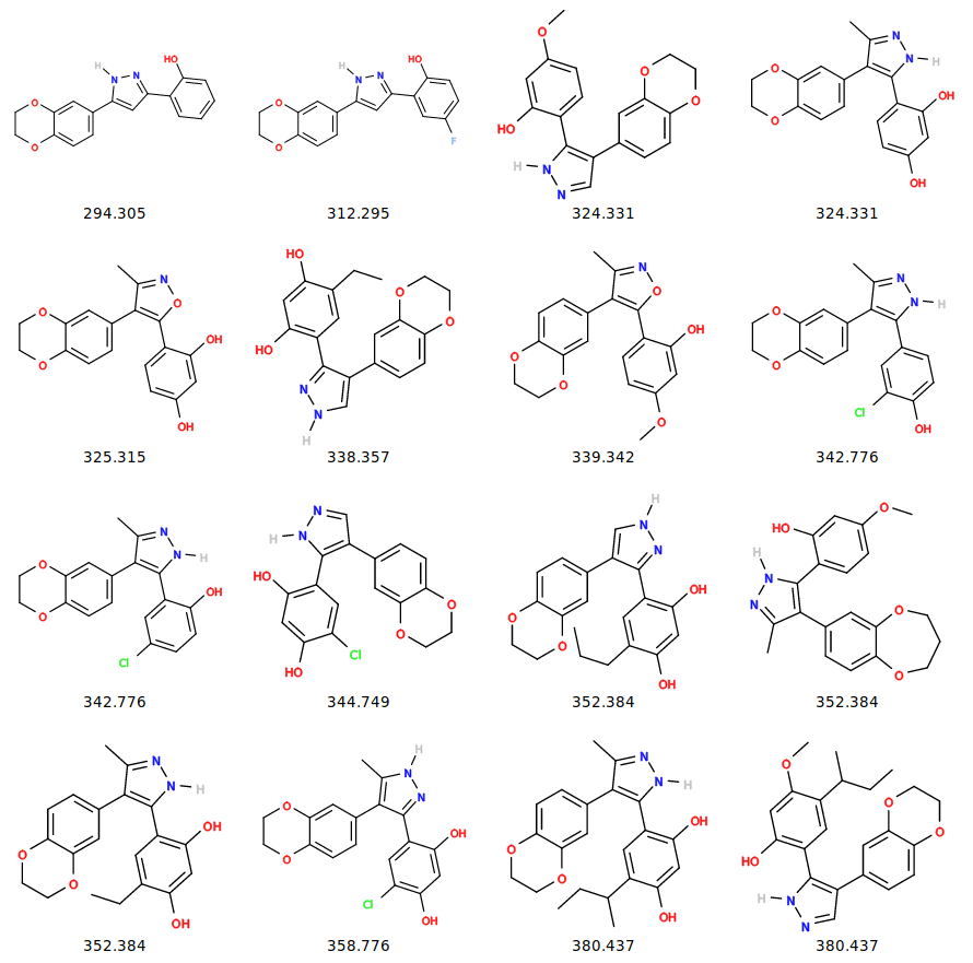
This produces an SVG image of all the structures generated ordered by molecular weight.
Figure 2: Structures of the compounds from ChEMBL.
Calculation of fingerprints and clustering
In this step, we will group similar molecules together. A key tool in cheminformatics for measuring molecular similarity is fingerprinting, which entails extracting chemical properties of molecules and storing them as a bitstring. These bitstrings can be easily compared computationally, for example with a clustering method. The fingerprinting tools in Galaxy are based on the Chemfp tools (Dalke 2013).
Before clustering, let’s label each compound. To do so add a second column to the SMILES compound library containing a label for each molecule. The Ligand SMILES file is also labelled something like /data/dnb02/galaxy_db/files/010/406/dataset_10406067.dat (the exact name will vary) and we would like to give it a more useful name. When labelling is complete, we can concatenate (join together) the library file with the original SMILES file for the ligand from the PDB file.
Hands-on: Calculate molecular fingerprints
ReplaceTool: toolshed.g2.bx.psu.edu/repos/bgruening/text_processing/tp_find_and_replace/1.1.3 with the following parameters:
param-file“File to process”: Ligand SMILES.
param-file“Find pattern”: add the current label of the SMILES here. You can find it by clicking the ‘view’ button next to the Ligand SMILES dataset - it will look something like /data/dnb02/galaxy_db/files/010/406/dataset_10406067.dat.
param-file“Replace with”: ligand
Concatenate datasetsTool: toolshed.g2.bx.psu.edu/repos/bgruening/text_processing/tp_cat/0.1.1 with the following parameters:
param-file“Datasets to concatenate”: Output of the previous step.
Click on Insert Dataset and in the new selection box which appears, select ‘Compound library’.
Run the step and rename the output dataset ‘Labelled compound library’.
Molecule to fingerprintTool: toolshed.g2.bx.psu.edu/repos/bgruening/chemfp/ctb_chemfp_mol2fps/1.5 with the following parameters:
param-file“Type of fingerprint”: Open Babel FP2 fingerprints
Rename to ‘Fingerprints’.
Taylor-Butina clustering (Butina 1999) provides a classification of the compounds into different groups or clusters, based on their structural similarity. This methods shows us how similar the compounds are to the original ligand, and after docking, we can compare the results to the proposed clusters to observe if there is any correlation.
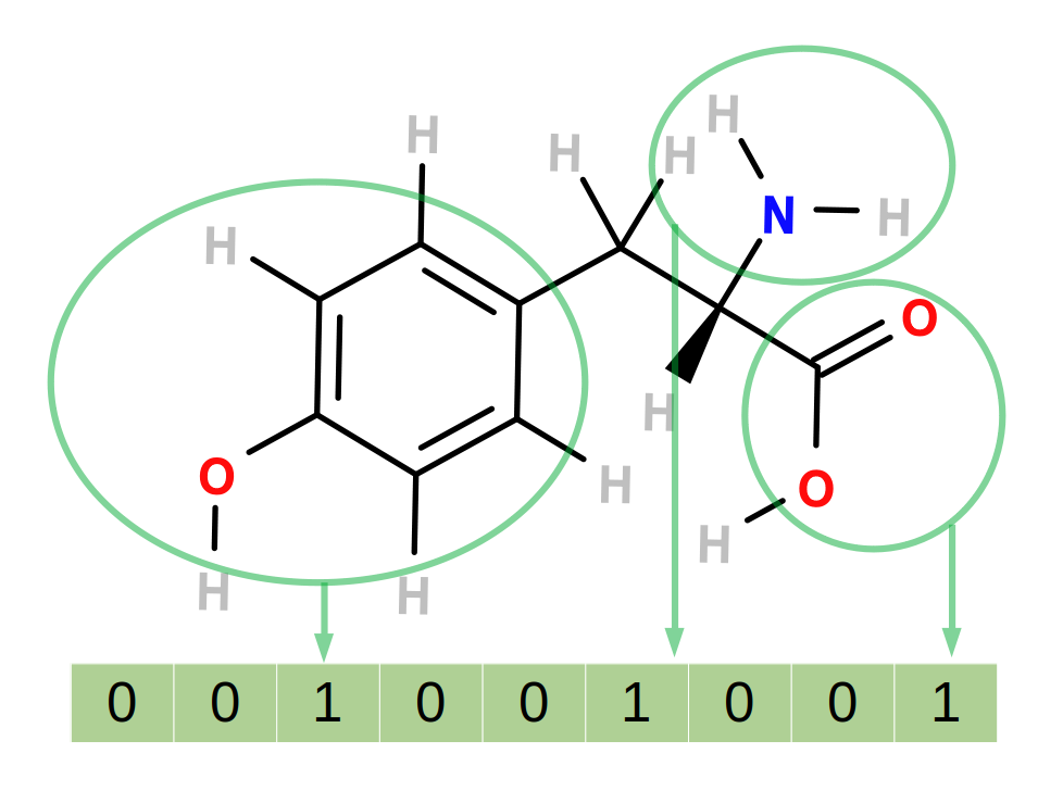
Figure 3: A simple fingerprinting system. Each 1 or 0 in the bitstring corresponds to the presence or absence of a particular feature in the molecule. In this case, the presence of phenyl, amine and carboxylic acid groups are encoded.
Hands-on: Cluster molecules using molecular fingerprints
Taylor-Butina clusteringTool: toolshed.g2.bx.psu.edu/repos/bgruening/chemfp/ctb_chemfp_butina_clustering/1.5 with the following parameters:
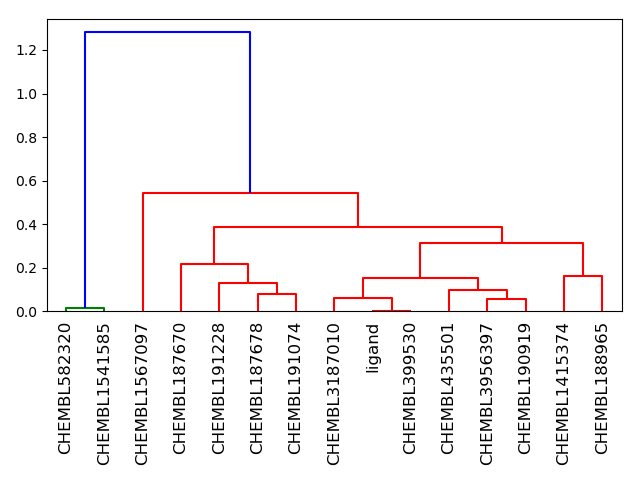
The image produced by the NxN clustering shows the clustering in the form of a dendrogram, where individual molecules are represented as vertical lines and merged into clusters. Merges are represented by horizontal lines. The y-axis represents the similarity of data points to each other; thus, the lower a cluster is merged, the more similar the data points are which it contains. Clusters in the dendogram are colored differently. For example, all molecules connected in red are similar enough to be grouped into the same cluster.
Figure 4: Dendrogram produced by NxN clustering. The library used to produce this image is generated with a Tanimoto cutoff of 80; here 15 search results are shown, plus the original ligand contained in the PDB file.
Try generating fingerprints using some of the other nine different protocols available and monitor how this affects the clustering.
For both the Taylor-Butina and NxN clustering, a threshold has to be set. Try varying this value and observe how the clustering results are affected.
Post-processing and plotting
From our collection of SD-files, we first extract all stored values into tabular format and then combine the files together to create a single tabular file.
Hands-on: Process SD-files
Extract values from an SD-fileTool: toolshed.g2.bx.psu.edu/repos/bgruening/sdf_to_tab/sdf_to_tab/2020.03.4+galaxy0 with the following parameters:
param-file“Input SD-file”: Collection of SD-files generated by the docking step. (Remember to select the ‘collection’ icon!)
param-file“Include the property name as header”: Yes
param-file“Include SMILES as column in output”: Yes
param-file“Include molecule name as column in output”: Yes
Leave all other paramters unchanged.
Collapse CollectionTool: toolshed.g2.bx.psu.edu/repos/nml/collapse_collections/collapse_dataset/4.2 with the following parameters:
param-file“Collection of files to collapse into single dataset”: Collection of tabular files generated by the previous step.
param-file“Keep one header line”: Yes
param-file“Append File name”: No
Click on param-collectionDataset collection in front of the input parameter you want to supply the collection to.
Select the collection you want to use from the list
Compound conversionTool: toolshed.g2.bx.psu.edu/repos/bgruening/openbabel_compound_convert/openbabel_compound_convert/3.1.1+galaxy0 with the following parameters:
param-file“Molecular input file”: choose one of the SD-files from the collection generated by the docking step.
param-file“Output format”: Protein Data Bank format (pdb)
param-file“Split multi-molecule files into a collection”: Yes
Leave all other parameters unchanged.
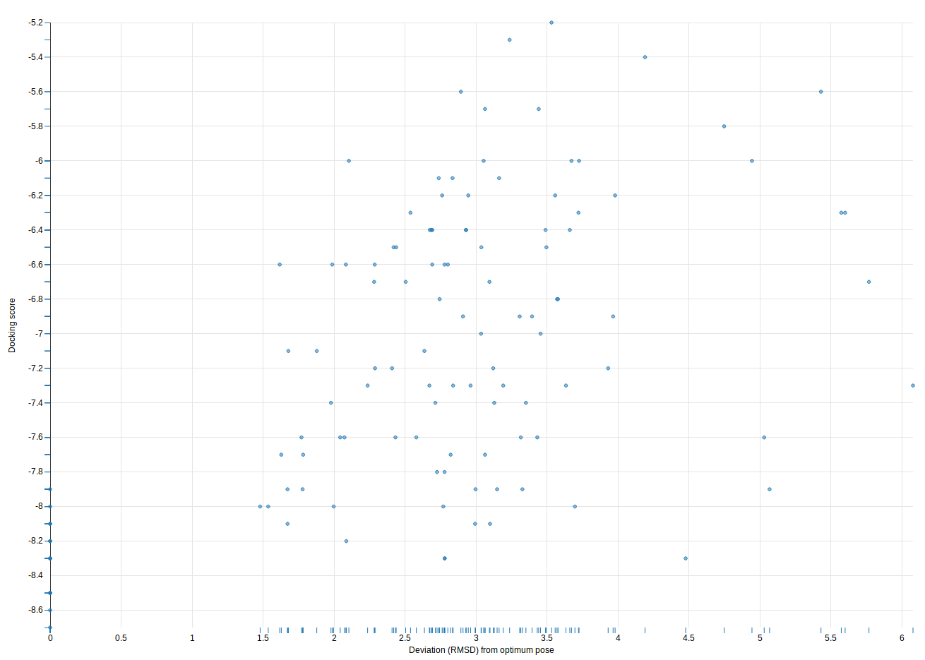
We now have a tabular file available which contains all poses calculated for all ligands docked, together with scores and RMSD values for the deviation of each pose from the optimum. We also have PDB files for some of the docking poses which can be inspected using the NGLViewer visualization embedded in Galaxy.
There are visualizations available in Galaxy for producing various types of plots - for example, a scatter plot of RMSD (compared to optimal docking pose) against docking score can be calculated very easily:
Figure 5: Scatter plot of RMSD against docking score.
The plot shows a correlation between the two variables, as expected, though only a slight one, given the narrow range of docking scores in the dataset and the structural similarity of the ligands tested.
A more advanced exercise would be to generate molecular descriptors for the molecule (there are three tools available for this in Galaxy: RDKit, Mordred and PaDEL) and to identify those which are particularly predictive of docking score, either by inspecting plots or using the statistics tools built into Galaxy.
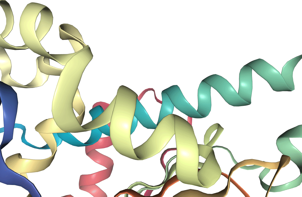
Use the NGLviewer to inspect the protein and various ligand poses generated by docking. This can be done using either the visualization of NGLViewer in Galaxy, or via the NGL website.
Figure 6: Two docking poses for a ligand bound to the active site of Hsp90. One (docking score -8.4) can be seen to be bound deeper in the active site than the other (docking score -5.7), which is reflected in the difference between the docking scores.
Key points
Docking allows ‘virtual screening’ of drug candidates
Molecular fingerprints encode features into a bitstring
The ChemicalToolbox contains many tools for cheminformatics analysis
Further information, including links to documentation and original publications, regarding the tools, analysis techniques and the interpretation of results described in this tutorial can be found here.
References
Humphrey, W., A. Dalke, and K. Schulten, 1996 VMD – Visual Molecular Dynamics. Journal of Molecular Graphics 14: 33–38. .
Butina, D., 1999 Unsupervised data base clustering based on daylight’s fingerprint and Tanimoto similarity: A fast and automated way to cluster small and large data sets. Journal of Chemical Information and Computer Sciences 39: 747–750.
Lipinski, C. A., 2004 Lead- and drug-like compounds: the rule-of-five revolution. Drug Discovery Today: Technologies 1: 337–341. 10.1016/j.ddtec.2004.11.007
Pearl, L. H., and C. Prodromou, 2006 Structure and Mechanism of the Hsp90 Molecular Chaperone Machinery. Annual Review of Biochemistry 75: 271–294. 10.1146/annurev.biochem.75.103004.142738
Le Guilloux, V., P. Schmidtke, and P. Tuffery, 2009 Fpocket: an open source platform for ligand pocket detection. BMC bioinformatics 10: 168.
Trott, O., and A. J. Olson, 2009 AutoDock Vina: Improving the speed and accuracy of docking with a new scoring function, efficient optimization, and multithreading. Journal of Computational Chemistry NA–NA. 10.1002/jcc.21334
O’Boyle, N. M., M. Banck, C. A. James, C. Morley, T. Vandermeersch et al., 2011 Open Babel: An open chemical toolbox. Journal of Cheminformatics 3: 10.1186/1758-2946-3-33
Dalke, A., 2013 The FPS fingerprint format and chemfp toolkit. Journal of cheminformatics 5: P36.
Gaulton, A., A. Hersey, M. Nowotka, Bento A Patrı́cia, J. Chambers et al., 2016 The ChEMBL database in 2017. Nucleic acids research 45: D945–D954.
Feedback
Did you use this material as an instructor? Feel free to give us feedback on how it went.
Did you use this material as a learner or student? Click the form below to leave feedback.
Batut et al., 2018 Community-Driven Data Analysis Training for Biology Cell Systems 10.1016/j.cels.2018.05.012
@misc{computational-chemistry-cheminformatics,
author = "Simon Bray",
title = "Protein-ligand docking (Galaxy Training Materials)",
year = "",
month = "",
day = ""
url = "\url{https://training.galaxyproject.org/training-material/topics/computational-chemistry/tutorials/cheminformatics/tutorial.html}",
note = "[Online; accessed TODAY]"
}
@article{Batut_2018,
    doi = {10.1016/j.cels.2018.05.012},
    url = {https://doi.org/10.1016%2Fj.cels.2018.05.012},
    year = 2018,
    month = {jun},
    publisher = {Elsevier {BV}},
    volume = {6},
    number = {6},
    pages = {752--758.e1},
    author = {B{\'{e}}r{\'{e}}nice Batut and Saskia Hiltemann and Andrea Bagnacani and Dannon Baker and Vivek Bhardwaj and Clemens Blank and Anthony Bretaudeau and Loraine Brillet-Gu{\'{e}}guen and Martin {\v{C}}ech and John Chilton and Dave Clements and Olivia Doppelt-Azeroual and Anika Erxleben and Mallory Ann Freeberg and Simon Gladman and Youri Hoogstrate and Hans-Rudolf Hotz and Torsten Houwaart and Pratik Jagtap and Delphine Larivi{\`{e}}re and Gildas Le Corguill{\'{e}} and Thomas Manke and Fabien Mareuil and Fidel Ram{\'{\i}}rez and Devon Ryan and Florian Christoph Sigloch and Nicola Soranzo and Joachim Wolff and Pavankumar Videm and Markus Wolfien and Aisanjiang Wubuli and Dilmurat Yusuf and James Taylor and Rolf Backofen and Anton Nekrutenko and Björn Grüning},
    title = {Community-Driven Data Analysis Training for Biology},
    journal = {Cell Systems}
}
Congratulations on successfully completing this tutorial!
 Simon Bray
 Questions: