You’ve done all the hard work of preparing a single cell matrix, processing it, plotting it, interpreting it, finding lots of lovely genes, all within the glorious Galaxy interface. Now you want to infer trajectories, or relationships between cells… and you’ve been threatened with learning Python to do so! Well, fear not. If you can have a run-through of a basic python coding introduction such as this one, then that will help you make more sense of this tutorial, however you’ll be able to make and interpret glorious plots even without understanding the Python coding language. This is the beauty of Galaxy - all the ‘set-up’ is identical across computers, because it’s browser based. So fear not!
Traditionally, we thought that differentiating or changing cells jumped between discrete states, so ‘Cell A’ became ‘Cell B’ as part of its maturation. However, most data shows otherwise, that generally there is a spectrum (a ‘trajectory’, if you will…) of small, subtle changes along a pathway of that differentiation. Trying to analyse cells every 10 seconds can be pretty tricky, so ‘pseudotime’ analysis takes a single sample and assumes that those cells are all on slightly different points along a path of differentiation. Some cells might be slightly more mature and others slightly less, all captured at the same ‘time’. We ‘assume’ or ‘infer’ relationships between cells.
We will use the same sample from the previous three tutorials, which contains largely T-cells in the thymus. We know T-cells differentiate in the thymus, so we would assume that we would capture cells at slightly different time points within the same sample. Furthermore, our cluster analysis alone showed different states of T-cell. Now it’s time to look further!
We’ve provided you with experimental data to analyse from a mouse dataset of fetal growth restriction Bacon et al. 2018. This is the full dataset generated from this tutorial (see the study in Single CellExpression Atlas here and the project submission here). You can find the final dataset in this input history or download from Zenodo below.
Open the Galaxy Upload Manager (galaxy-upload on the top-right of the tool panel)
Select Paste/Fetch Data
Paste the link into the text field
Press Start
Close the window
Renamegalaxy-pencil the .h5ad object as Final cell annotated object
Click on the galaxy-pencilpencil icon for the dataset to edit its attributes
In the central panel, change the Name field to Final cell annotated object
Click the Save button
Check that the datatype is h5ad
Click on the galaxy-pencilpencil icon for the dataset to edit its attributes
In the central panel, click on the galaxy-chart-select-dataDatatypes tab on the top
Select h5ad
tip: you can start typing the datatype into the field to filter the dropdown menu
Click the Save button
Renamegalaxy-pencil the .ipynb object as Trajectories_Instructions.ipynb
Check that the datatype is .ipynb
Filtering for T-cells
One problem with our current dataset is that it’s not just T-cells: we found in the previous tutorial that it also contains macrophages. This is a problem, because trajectory analysis will generally try to find relationships between all the cells in the sample. We need to remove those cell types to analyse the trajectory.
Tools are frequently updated to new versions. Your Galaxy may have multiple versions of the same tool available. By default, you will be shown the latest version of the tool. This may NOT be the same tool used in the tutorial you are accessing. Furthermore, if you use a newer tool in one step, and try using an older tool in the next step… this may fail! To ensure you use the same tool versions of a given tutorial, use the Tutorial mode feature.
Open your Galaxy server
Click on the curriculum icon on the top menu, this will open the GTN inside Galaxy.
Navigate to your tutorial
Tool names in tutorials will be blue buttons that open the correct tool for you
Note: this does not work for all tutorials (yet)
You can click anywhere in the grey-ed out area outside of the tutorial box to return back to the Galaxy analytical interface
Hands-on: Removing macrophages
Manipulate AnnDataTool: toolshed.g2.bx.psu.edu/repos/iuc/anndata_manipulate/anndata_manipulate/0.7.5+galaxy1 with the following parameters:
param-file“Annotated data matrix”: Final cell annotated object
“Function to manipulate the object”: Filter observations or variables
You should now have 8569 cells, as opposed to the 8605 you started with. You’ve only removed a few cells (the contaminants!), but it makes a big difference in the next steps.
Take note of what # this dataset is in your history, as you will need that shortly!
Launching Jupyter
Warning: Data uploads and Jupyter
There are a few ways of importing and uploading data in Jupyter. You might find yourself accidentally doing this differently than the tutorial, and that’s ok. There are a few key steps where you will call files from a location - if these don’t work from you, check that the file location is correct and change accordingly!
JupyterLab is a bit like RStudio but for other coding languages. What, you’ve never heard of RStudio? Then don’t worry, just follow the instructions!
You will need to download the tutorial notebook locally to your own computer. Do this by going here: Download the notebook
Hands-on: Launching JupyterLab
Interactive JupyTool and NotebookTool: interactive_tool_jupyter_notebook with the following parameters:
“Do you already have a notebook?”: Start with a fresh notebook
This may take a moment, but once the Executed notebook in your dataset is orange, you are up and running!
Either click on the blue User menu, or go to the top of the screen and choose User and then Active InteractiveTools
Click on the newest JupyTool interactive tool.
Welcome!
Warning: Danger: You can lose data!
Do NOT delete or close this notebook dataset in your history. YOU WILL LOSE IT!
Hands-on: Creating a notebook
Click the Python 3 icon under Notebook
Figure 1: Python 3 Button
Save your file (File: Save, or click the galaxy-save Save icon at the top left)
If you right click on the file in the folder window at the left, you can rename your file whateveryoulike.ipynb
Cool! Now you know how to create a file! Helpfully, however, we have created one for you, and you’ve downloaded it onto your computer already!
Hands-on: Uploading the tutorial notebook
In the folder window, galaxy-upload Upload the Trajectories_Instructions.ipynb from your computer. It should appear in the file window.
Open it by double clicking it in the file window.
Warning: You should Save frequently!
This is both for good practice and to protect you in case you accidentally close the browser. Your environment will still run, so it will contain the last saved notebook you have. You might eventually stop your environment after this tutorial, but ONLY once you have saved and exported your notebook (more on that at the end!) Note that you can have multiple notebooks going at the same time within this JupyterLab, so if you do, you will need to save and export each individual notebook. You can also download them at any time.
Run the tutorial!
At this point, to prevent you having to switch back and forth between browsers, the directions for the rest of tutorial are all in the notebook you input! You may have to change certain numbers in the code blocks, so do read carefully. You will be able to run each step be clicking on the code block and pressing the workflow-runRun the selected cells and advance step. You will want to keep a tab open with your Galaxy history showing (so just launch another browser of your usegalaxy.eu instance), so that you can see when your files appear there. The tutorial is adapted from the Scanpy Trajectory inference tutorial.
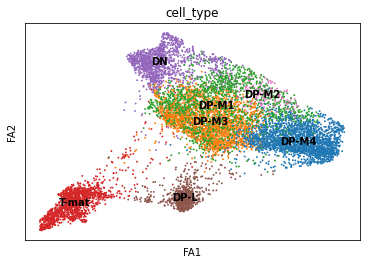
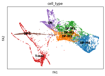
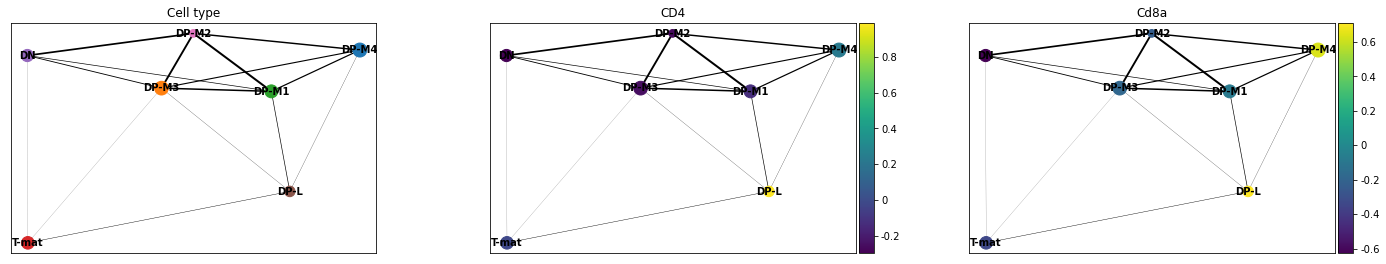
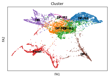
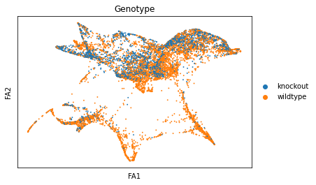
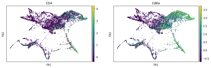
Tutorial Plot Answers
Just in case, we’ve put the plots you should generate in the tutorial here. If things have gone wrong, you can also download this answer key tutorial.
congratulations Congratulations! You’ve made it through Jupyter!
Hands-on: Closing JupyterLab
Click User: Active Interactive Tools
Tick galaxy-selector the box of your Jupyter Interactive Tool, and click Stop
If you want to run this notebook again, or share it with others, it now exists in your history. You can use this ‘finished’ version just the same way as you downloaded the directions file and uploaded into the Jupyter environment.
In this tutorial, you moved from called clusters to inferred relationships and trajectories using pseudotime analysis. You found an alternative to PCA (diffusion map), an alternative to tSNE (force-directed graph), a means of identifying cluster relationships (PAGA), and a metric for pseudotime (diffusion pseudotime) to identify early and late cells. If you were working in a group, you found that such analysis is slightly more sensitive to your decisions than the simpler filtering/plotting/clustering is. We are inferring and assuming relationships and time, so that makes sense!
To discuss with like-minded scientists, join our Gitter channel for all things Galaxy-single cell!
Key points
Trajectory analysis is less robust than pure plotting methods, as such ‘inferred relationships’ are a bigger mathematical leap
As always with single-cell analysis, you must know enough biology to deduce if your analysis is reasonable, before exploring or deducing novel insight
Further information, including links to documentation and original publications, regarding the tools, analysis techniques and the interpretation of results described in this tutorial can be found here.
References
Bacon, W. A., R. S. Hamilton, Z. Yu, J. Kieckbusch, D. Hawkes et al., 2018 Single-Cell Analysis Identifies Thymic Maturation Delay in Growth-Restricted Neonatal Mice. Frontiers in Immunology 9: 10.3389/fimmu.2018.02523
Feedback
Did you use this material as an instructor? Feel free to give us feedback on how it went.
Did you use this material as a learner or student? Click the form below to leave feedback.
Batut et al., 2018 Community-Driven Data Analysis Training for Biology Cell Systems 10.1016/j.cels.2018.05.012
@misc{transcriptomics-scrna-case_JUPYTER-trajectories,
author = "Wendi Bacon and Mehmet Tekman",
title = "Inferring Trajectories using Python (Jupyter Notebook) in Galaxy (Galaxy Training Materials)",
year = "",
month = "",
day = ""
url = "\url{https://training.galaxyproject.org/training-material/topics/transcriptomics/tutorials/scrna-case_JUPYTER-trajectories/tutorial.html}",
note = "[Online; accessed TODAY]"
}
@article{Batut_2018,
    doi = {10.1016/j.cels.2018.05.012},
    url = {https://doi.org/10.1016%2Fj.cels.2018.05.012},
    year = 2018,
    month = {jun},
    publisher = {Elsevier {BV}},
    volume = {6},
    number = {6},
    pages = {752--758.e1},
    author = {B{\'{e}}r{\'{e}}nice Batut and Saskia Hiltemann and Andrea Bagnacani and Dannon Baker and Vivek Bhardwaj and Clemens Blank and Anthony Bretaudeau and Loraine Brillet-Gu{\'{e}}guen and Martin {\v{C}}ech and John Chilton and Dave Clements and Olivia Doppelt-Azeroual and Anika Erxleben and Mallory Ann Freeberg and Simon Gladman and Youri Hoogstrate and Hans-Rudolf Hotz and Torsten Houwaart and Pratik Jagtap and Delphine Larivi{\`{e}}re and Gildas Le Corguill{\'{e}} and Thomas Manke and Fabien Mareuil and Fidel Ram{\'{\i}}rez and Devon Ryan and Florian Christoph Sigloch and Nicola Soranzo and Joachim Wolff and Pavankumar Videm and Markus Wolfien and Aisanjiang Wubuli and Dilmurat Yusuf and James Taylor and Rolf Backofen and Anton Nekrutenko and Björn Grüning},
    title = {Community-Driven Data Analysis Training for Biology},
    journal = {Cell Systems}
}
Congratulations on successfully completing this tutorial!
 Wendi Bacon
 Mehmet Tekman

 Helena Rasche
 Julia Jakiela
 Questions: