Introduction

What is a microbiome? It is a collection of small living creatures. These small creatures are called micro-organisms and they are everywhere. In our gut, in the soil, on vending machines, and even inside the beer. Most of these micro-organisms are actually very good for us, but some can make us very ill.

Micro-organisms come in different shapes and sizes, but they have the same components. One crucial component is the DNA, the blueprint of life. The DNA encodes the shape and size and many other characteristics unique to a species. Because DNA is so species-specific, reading the DNA can be used to identify what kind of micro-organism the it is from. Therefore, within a metagenomic specimen, e.g. a sample form soil, gut, or beer, one can identify what kind of species are inside the sample.

In this tutorial, we will use data of beer microbiome generated via the BeerDEcoded project.

Details: The BeerDEcoded project

The BeerDEcoded Project is a series of workshops organized with and for schools as well as the general audience, aiming to introduce biology and genomic science. People learn in an interactive way about DNA, sequencing technologies, bioinformatics, open science, how these technologies and concepts are applied and how they are impacting their daily life.

Beer is alive and contains many microorganisms. It can be found in many places and there are many of them. It is a fun media to bring the people to the contact of molecular biology, data-analysis, and open science.

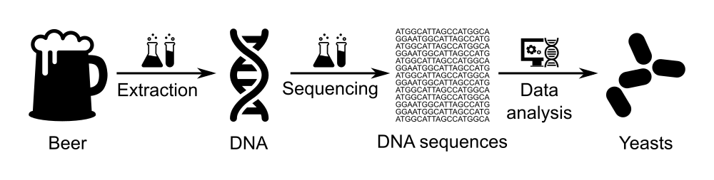
A BeerDEcoded workshop includes the following steps:

1. Extract yeasts and their DNA from beer bottle,
2. Sequence the extracted DNA using a MinION sequencer to obtain the sequence of bases/nucleotides (A, T, C and G) for each DNA fragment in the sample,
3. Analyze the sequenced data in order to know which organisms this DNA is from

Comment: Beer microbiome

Beer is alive! It contains microorganisms, in particular yeasts.

Indeed, grain and water create a sugary liquid (called wort). The beer brewer adds yeasts to it. By eating the sugar, yeasts creates alcohol, and other compounds (esters, phenols, etc.) that give beer its particular flavor.

Yeasts are microorganisms, more precisely unicellular fungi. The majority of beers use a yeast genus called Saccharomyces, which in Greek means “sugar fungus”. Within that genus, two specific species of Saccharomyces are the most commonly used:

• Saccharomyces cerevisiae: a top-fermenting (i.e. yeast which rise up to the top of the beer as it metabolizes sugars, delivering alcohol as a by-product), ale yeast responsible for a huge range of beer styles like witbiers, stouts, ambers, tripels, saisons, IPAs, and many more. It is most likely the yeast that the early brewers were inadvertently brewing with over 3,000 years ago.
• Saccharomyces pastorianus: a bottom-fermenting (i.e. it sits on the bottom of the tank as it ferments) lager yeast, responsible for beer styles like Pilsners, lagers, märzens, bocks, and more. This yeast was originally found, and cultivated, by Bavarian brewers a little over 200 years ago. It is the most commonly used yeast in terms of the raw amount of beer produced around the world.

But yeast is actually all around us. And we can actually brew spontaneously fermented beer with wild yeast and souring microbiota floating through the air.

During one BeerDEcoded workshop, we extracted yeasts out of a bottle of Chimay. We then extracted the DNA of these yeasts and sequenced it using a MinION to obtain the DNA sequences. Now, we would like to identify the yeast species sequenced there, and thereby outline the diversity of microorganisms (the microbiome community) in the beer sample.

To get this information, we need to process the sequenced data in a few steps:

1. Check the quality of the data
2. Assign a taxonomic label, i.e. assign ‘species’ to each sequence
3. Visualize the distribution of the different species

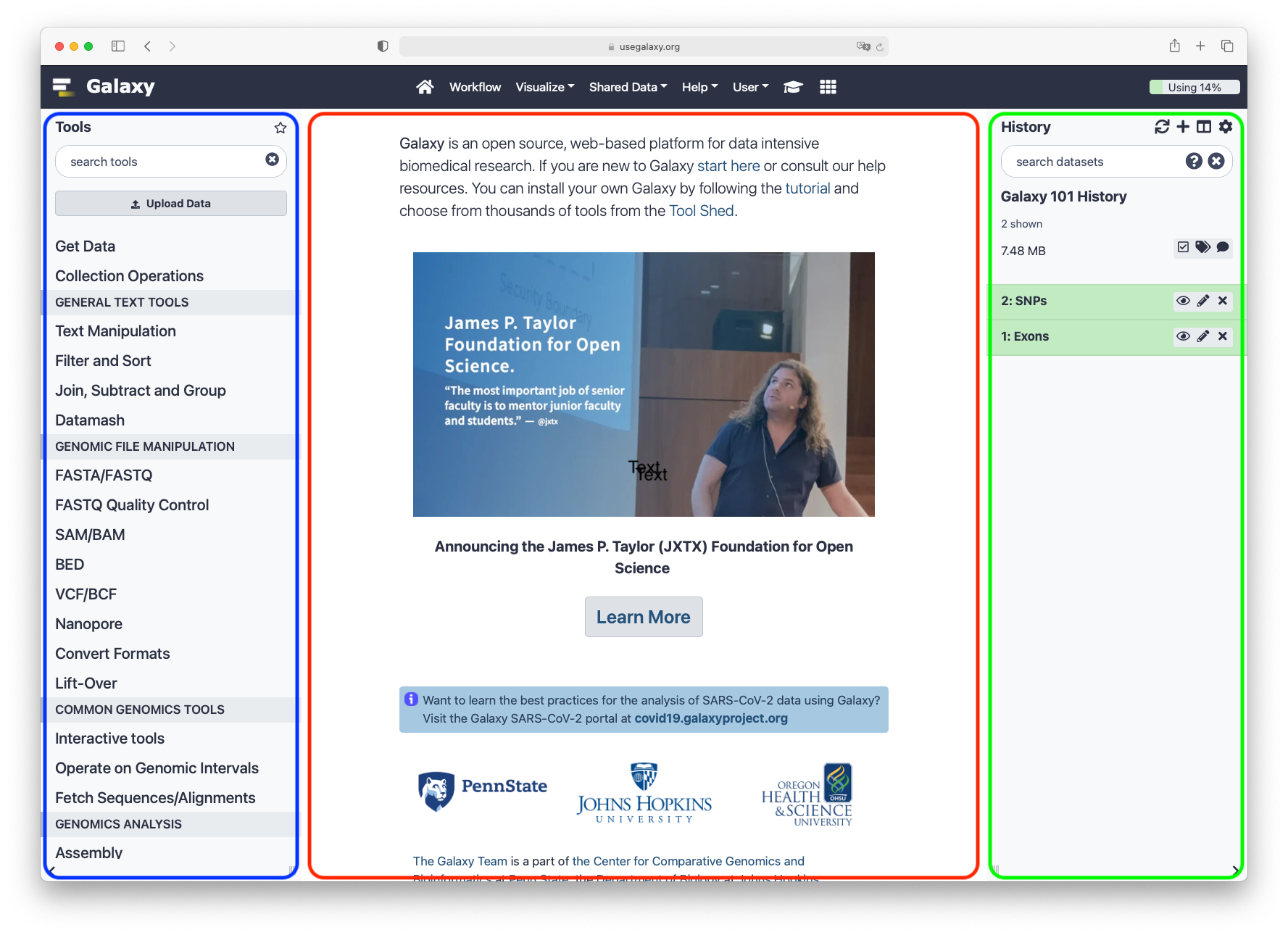
This type of data analysis requires running several bioinformatics tools and usually requires a computer science background. Galaxy is an open-source platform for data analysis that enables anyone to use bioinformatics tools through its graphical web interface, accessible via any Web browser.

So, in this tutorial, we will use Galaxy to extract and visualize the community of yeasts from a bottle of beer.

Agenda

In this tutorial, we will cover:

1. Introduction
2. Prepare Galaxy and data
   1. Get familiar with Galaxy
   2. Get data
3. Data quality
   1. Assess data quality
   2. Improve the dataset quality
4. Assign taxonomic classification
5. Visualize the community
6. (Optional) Sharing your history

Prepare Galaxy and data

First of all, this tutorial will get you hands on with some basic Galaxy tasks, including creating a history and importing data.

Get familiar with Galaxy

Hands-on: Open Galaxy

1. Open your favorite browser (Works on Chrome, Firefox, Safari but not Internet Explorer!)

2. Create a Galaxy account if you do not have one

   Tip: How do I create an account on a public Galaxy instance?

   1. To create an account at any public Galaxy instance, choose your server from the available list of Galaxy Platform.

      There are 3 main public Galaxy servers: UseGalaxy.org, UseGalaxy.eu, and UseGalaxy.org.au.

   2. Click on “Login or Register” in the masthead on the server.

      

   3. Click on Register here and fill in the required information.
   4. Click on the Create button, your account is successfully created.
   5. Check for a Confirmation Email in the email you used for account creation.
   6. Click on the Email confirmation link to fully activate your account.

The Galaxy homepage is divided into three panels:

• Tools on the left
• Viewing panel in the middle
• History of analysis and files on the right

The first time you use Galaxy, there will be no files in your history panel.

Any analysis should get its own Galaxy history. So let’s start by creating a new one:

Hands-on: Prepare the Galaxy history

1. Create a new history for this analysis

   Tip: Creating a new history

   Click the new-history icon at the top of the history panel.

   If the new-history is missing:

   1. Click on the galaxy-gear icon (History options) on the top of the history panel
   2. Select the option Create New from the menu

2. Rename the history

   Tip: Renaming a history

   1. Click on Unnamed history (or the current name of the history) (Click to rename history) at the top of your history panel
   2. Type the new name
   3. Press Enter

Get data

Before we can begin any Galaxy analysis, we need to upload the input data: FASTQ files

Hands-on: Upload your dataset

1. Import the sequenced data including fastq in the name

   • Option 1 video: Your own local data using Upload Data (recommended for 1-10 datasets).

     Tip: Upload few files (1-10)

     1. Click on Upload Data on the top of the left panel
     2. Click on Choose local file and select the files or drop the files in the Drop files here part
     3. Click on Start
     4. Click on Close

   • Option 2: From Zenodo, an external server, via URL

     https://zenodo.org/record/7093173/files/ABJ044_c38189e89895cdde6770a18635db438c8a00641b.fastq
     

     Tip: Importing via links

     • Copy the link location

     • Open the Galaxy Upload Manager (galaxy-upload on the top-right of the tool panel)

     • Select Paste/Fetch Data

     • Paste the link into the text field

     • Press Start

     • Close the window

   Your uploaded file is now in your current history. When the file is fully uploaded to Galaxy, it will turn green. But, what is this file?

2. Click on the galaxy-eye (eye) icon next to the dataset name to look at the file contents.

The contents of the file will be displayed in the central Galaxy panel.

This file contains the sequences, also called reads, of DNA, i.e. succession of nucleotides, for all fragments from the yeasts in the beer, in FASTQ format.

Details: FASTQ format

Although it looks complicated (and maybe it is), the FASTQ format is easy to understand with a little decoding. Each read, representing a fragment of DNA, is encoded by 4 lines:

Line	Description
1	Always begins with @ followed by the information about the read
2	The actual nucleic sequence
3	Always begins with a + and contains sometimes the same info in line 1
4	Has a string of characters which represent the quality scores associated with each base of the nucleic sequence; must have the same number of characters as line 2

So for example, the first sequence in our file is:

@03dd2268-71ef-4635-8bce-a42a0439ba9a runid=8711537cc800b6622b9d76d9483ecb373c6544e5 read=252 ch=179 start_time=2019-12-08T11:54:28Z flow_cell_id=FAL10820 protocol_group_id=la_trappe sample_id=08_12_2019
AGTAAGTAGCGAACCGGTTTCGTTTGGGTGTTTAACCGTTTTCGCATTTATCGTGAAACGCTTTCGCGTTTTCGTGCGGAAGGCGCTTCACCCAGGGCCTCTCATGCTTTGTCTTCCTGTTTATTCAGGATCGCCCAAAGCGAGAATCATACCACTAGACCACACGCCCGAATTATTGTTGCGTTAATAAGAAAAGCAAATATTTAAGATAGGAAGTGATTAAAGGGAATCTTCTACCAACAATATCCATTCAAATTCAGGCA
+
$'())#$$%#$%%'-$&$%'%#$%('+;<>>>18.?ACLJM7E:CFIMK<=@0/.4<9<&$007:,3<IIN<3%+&$(+#$%'$#$.2@401/5=49IEE=CH.20355>-@AC@:B?7;=C4419)*$$46211075.$%..#,529,''=CFF@:<?9B522.(&%%(9:3E99<BIL?:>RB--**5,3(/.-8B>F@@=?,9'36;:87+/19BAD@=8*''&''7752'$%&,5)AM<99$%;EE;BD:=9<@=9+%$

It means that the fragment named @03dd2268-71ef-4635-8bce-a42a0439ba9a (ID given in line1) corresponds to:

• the DNA sequence AGTAAGTAGCGAACCGGTTTCGTTTGGGTGTTTAACCGTTTTCGCATTTATCGTGAAACGCTTTCGCGTTTTCGTGCGGAAGGCGCTTCACCCAGGGCCTCTCATGCTTTGTCTTCCTGTTTATTCAGGATCGCCCAAAGCGAGAATCATACCACTAGACCACACGCCCGAATTATTGTTGCGTTAATAAGAAAAGCAAATATTTAAGATAGGAAGTGATTAAAGGGAATCTTCTACCAACAATATCCATTCAAATTCAGGCA (line2)
• this sequence has been sequenced with a quality $'())#$$%#$%%'-$&$%'%#$%('+;<>>>18.?ACLJM7E:CFIMK<=@0/.4<9<&$007:,3<IIN<3%+&$(+#$%'$#$.2@401/5=49IEE=CH.20355>-@AC@:B?7;=C4419)*$$46211075.$%..#,529,''=CFF@:<?9B522.(&%%(9:3E99<BIL?:>RB--**5,3(/.-8B>F@@=?,9'36;:87+/19BAD@=8*''&''7752'$%&,5)AM<99$%;EE;BD:=9<@=9+%$ (line 4).

But what does this quality score mean?

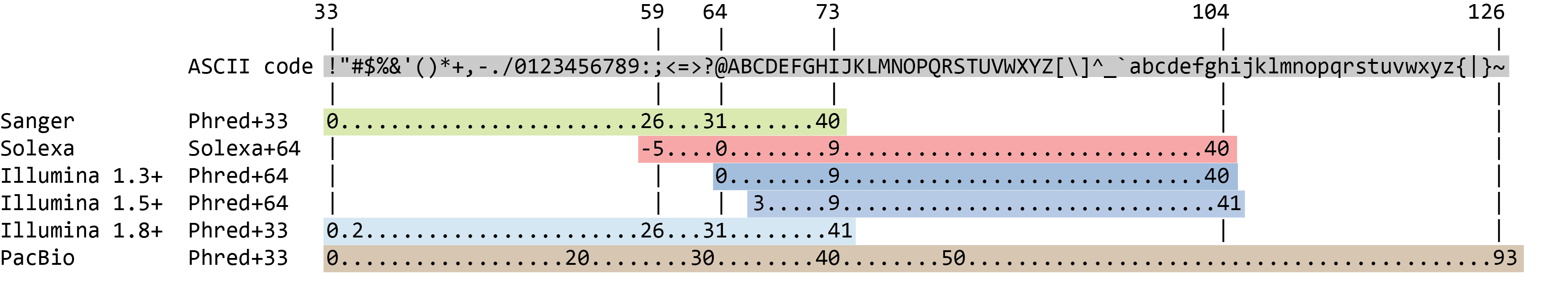
The quality score for each sequence is a string of characters, one for each base of the nucleotide sequence, used to characterize the probability of misidentification of each base. The score is encoded using the ASCII character table (with some historical differences):

So there is an ASCII character associated with each nucleotide, representing its Phred quality score, the probability of an incorrect base call:

Phred Quality Score	Probability of incorrect base call	Base call accuracy
10	1 in 10	90%
20	1 in 100	99%
30	1 in 1000	99.9%
40	1 in 10,000	99.99%
50	1 in 100,000	99.999%
60	1 in 1,000,000	99.9999%

Data quality

Assess data quality

Before starting to work on our data, it is necessary to assess its quality. This is an essential step if we aim to obtain a meaningful downstream analysis.

FastQC is one of the most widely used tools to check the quality of data generated by High Throughput Sequencing (HTS) technologies.

Hands-on: Quality check

1. FASTQC Tool: toolshed.g2.bx.psu.edu/repos/devteam/fastqc/fastqc/0.73+galaxy0 with the following parameters
   • param-file “Raw read data from your current history”: Reads
2. Inspect the generated HTML file

Question

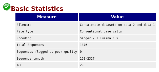
Given the Basic Statistics table on the top of the page:

1. How many sequences are in the FASTQ file?
2. How long are the sequences?

Solution

1. There are 1876 sequences.
2. The sequences range from 130 nucleotides to 2327 nucleotides. Not all sequences have then the same length.

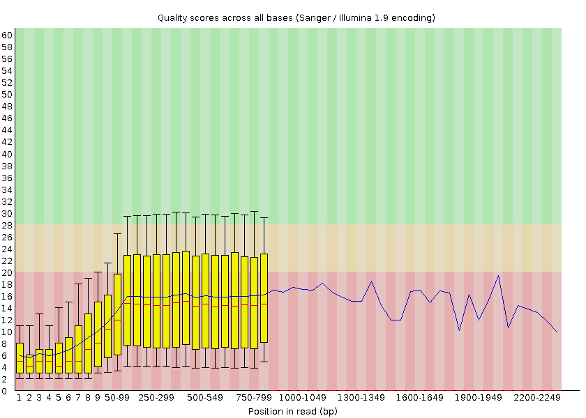
FastQC provides information on various parameters, such as the range of quality values across all bases at each position:

We can see that the quality of our sequencing data grows after the first few bases, stays around a score of 18 and then decreases again at the end of the sequences. MinION and Oxford Nanopore Technologies (ONT) are known to have a higher error rate compared to other sequencing techniques and platforms (Delahaye and Nicolas 2021).

For more detailed information about the other plots in the FASTQC report, check out our dedicated tutorial.

Improve the dataset quality

In order to improve the quality of our data, we will use two tools:

• porechop (Wick 2017) to remove adapters that were added for sequencing and chimera (contaminant)
• fastp (Chen et al. 2018) to filter sequences with low quality scores (below 10)

Hands-on: Improve the dataset quality

1. Porechop Tool: toolshed.g2.bx.psu.edu/repos/iuc/porechop/porechop/0.2.3 with the following parameters:
   • param-file “Input FASTA/FASTQ”: Reads
   • “Output format for the reads”: fastq
2. fastp Tool: toolshed.g2.bx.psu.edu/repos/iuc/fastp/fastp/0.23.2+galaxy0 with the following parameters:
   • “Single-end or paired reads”: Single-end
   • param-file “Dataset collection”: output of Porechop
   • In “Adapter Trimming Options”:
     • “Disable adapter trimming”: Yes
   • In “Filter Options”:
     • In “Quality filtering options”:
       • “Qualified quality phred”: 10
   • In “Read Modification Options”:
     • “PolyG tail trimming”: Disable polyG tail trimming
3. Inspect the HTML report of fastp to see how the quality has been improved

Question

1. How many sequences are there before filtering? Is it the same number as in FASTQC report?
2. How many sequences are there after filtering? How many sequences have then been removed by filtering?
3. What is the mean length before filtering? And after filtering?

Solution

1. There are 1,869 reads before filtering. The number is lower than in the FASTQC report. Some reads may have been discarded via Porechop
2. There are 1,350 reads after filtering. So the filtering step has removed \(1869-1350 = 519\) sequences.
3. The mean length is 314 nucleotide before filtering and 316bp after filtering.

Assign taxonomic classification

One of the main aims in microbiome data analysis is to identify the organisms sequenced. For that we try to identify the taxon to which each individual reads belong.

Details: What is Taxonomy?

Taxonomy is the method used to naming, defining (circumscribing) and classifying groups of biological organisms based on shared characteristics such as morphological characteristics, phylogenetic characteristics, DNA data, etc. It is founded on the concept that the similarities descend from a common evolutionary ancestor.

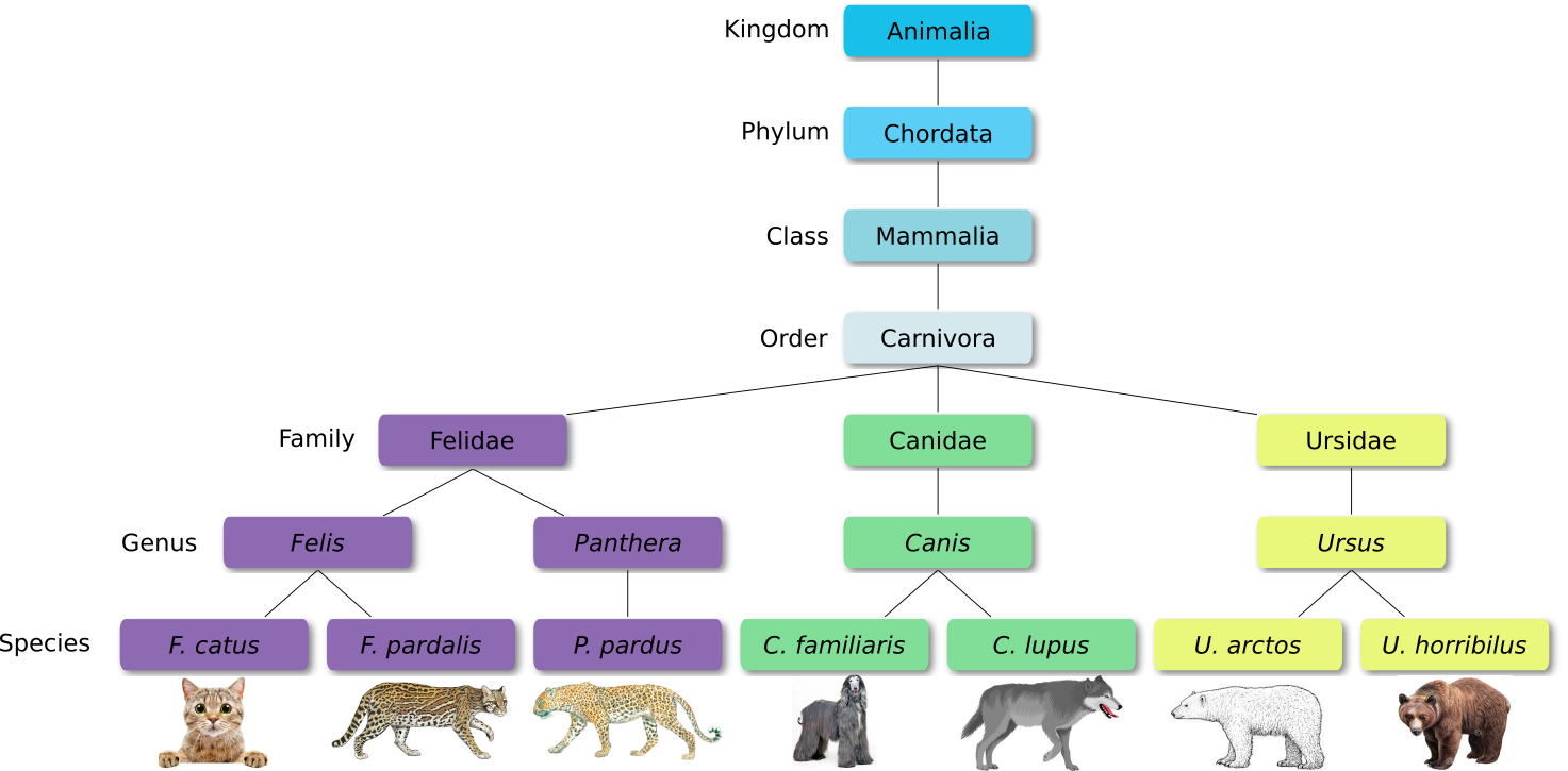
Defined groups of organisms are known as taxa. Taxa are given a taxonomic rank and are aggregated into super groups of higher rank to create a taxonomic hierarchy. The taxonomic hierarchy includes eight levels: Domain, Kingdom, Phylum, Class, Order, Family, Genus and Species.

The classification system begins with 3 domains that encompass all living and extinct forms of life

• The Bacteria and Archae are mostly microscopic, but quite widespread.
• Domain Eukarya contains more complex organisms

When new species are found, they are assigned into taxa in the taxonomic hierarchy. For example for the cat:

Level	Classification
Domain	Eukaryota
Kingdom	Animalia
Phylum	Chordata
Class	Mammalia
Order	Carnivora
Family	Felidae
Genus	Felis
Species	F. catus

Let’s explore taxonomy in the Tree of Life, using Lifemap

Question

1. Which microorganisms do we expect to identify in our data?
2. What is the taxonomy of main expected microorganism?

Solution

1. The sequences are supposed to be yeasts extracted from a bottle of beer. The majority of beers contain a yeast genus called Saccharomyces and 2 species in that genus: Saccharomyces cerevisiae (ale yeast) and Saccharomyces pastorianus (lager yeast). The used beer is an ale beer, so we expect to find Saccharomyces cerevisiae. But other yeasts can also have been used and then found. We could also have some DNA left from other beer components, but also contaminations by other microorganisms and even human DNA from people who manipulated the beer or did the extraction.

2. The main expected microorganism is Saccharomyces cerevisiae with its taxonomy:

   Level	Classification
   Domain	Eukaryota
   Kingdom	Fungi
   Phylum	Ascomycota
   Class	Saccharomycetes
   Order	Saccharomycetales
   Family	Saccharomycetaceae
   Genus	Saccharomyces
   Species	S. cerevisiae

Taxonomic assignment or classification is the process of assigning an Operational Taxonomic Unit (OTUs, that is, groups of related individuals / taxon) to sequences. To assign an OTU to a sequence it is compared against a database, but this comparison can be done in different ways, with different bioinformatics tools. Here we will use Kraken2 (Wood et al. 2019).

Details: Kraken2 and the k-mer approach for taxonomy classification

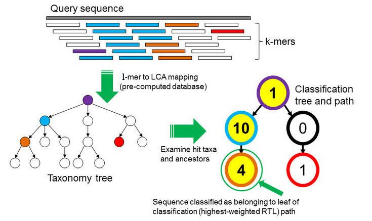
In the \(k\)-mer approach for taxonomy classification, we use a database containing DNA sequences of genomes whose taxonomy we already know. On a computer, the genome sequences are broken into short pieces of length \(k\) (called \(k\)-mers), usually 30bp.

Kraken examines the \(k\)-mers within the query sequence, searches for them in the database, looks for where these are placed within the taxonomy tree inside the database, makes the classification with the most probable position, then maps \(k\)-mers to the lowest common ancestor (LCA) of all genomes known to contain the given \(k\)-mer.

Hands-on: Kraken2

1. Kraken2 Tool: toolshed.g2.bx.psu.edu/repos/iuc/kraken2/kraken2/2.0.8_beta+galaxy0 with the following parameters:
   • “Single or paired reads”: Single
     • param-file “Input sequences”: Output of fastp
   • “Print scientific names instead of just taxids”: Yes
   • In “Create Report”:
     • “Print a report with aggregrate counts/clade to file”: Yes
     • “Format report output like Kraken 1’s kraken-mpa-report”: Yes

   • “Select a Kraken2 database”: Prebuilt Refseq indexes: PlusPF

     The database here contains reference sequences and taxonomies. We need to be sure it contains yeasts, i.e. fungi.

2. Inspect the report file

The Kraken report in MPA format is a tabular file with 2 columns:

d__Eukaryota	756
d__Eukaryota|k__Metazoa	402
d__Eukaryota|k__Metazoa|p__Chordata	402
d__Eukaryota|k__Metazoa|p__Chordata|c__Mammalia	402
d__Eukaryota|k__Metazoa|p__Chordata|c__Mammalia|o__Primates	402
d__Eukaryota|k__Metazoa|p__Chordata|c__Mammalia|o__Primates|f__Hominidae	402
d__Eukaryota|k__Metazoa|p__Chordata|c__Mammalia|o__Primates|f__Hominidae|g__Homo	402
d__Eukaryota|k__Metazoa|p__Chordata|c__Mammalia|o__Primates|f__Hominidae|g__Homo|s__Homo sapiens	402
d__Eukaryota|k__Fungi	342
d__Eukaryota|k__Fungi|p__Ascomycota	341
d__Eukaryota|k__Fungi|p__Ascomycota|c__Saccharomycetes	336
...

1. The first column lists clades, ranging from taxonomic domains (Bacteria, Archaea, etc.) through species.

   The taxonomic level of each clade is prefixed to indicate its level:

   • Domain: d__
   • Kingdom: k__
   • Phylum: p__
   • Class: c__
   • Order: o__
   • Family: f__
   • Genus: g__
   • Species: s__

2. The second column gives the number of reads assigned to the clade rooted at that taxon

Question

1. How many taxons have been identified?
2. How many reads have been classified?
3. Which domains were found and with how many reads?
4. Which yeasts have been identified? Are they the expected ones?

Solution

1. The file contains 215 lines (information visible when expanding the report dataset in the history panel). So 215 taxons have been identified.

2. On the 1350 sequences in the input, 837 (62%) were classified (or identified as a taxon) and 513 unclassified (38%). Information visible when expanding the report dataset in the history panel, and scrolling in the small box starting with “Loading database information” below the format information.

3. The 3 domains were found:
   • Eukaryota with 756 reads assigned to it
   • Bacteria with 17 reads
   • Archaea with 2 reads

4. Yeasts do not form a single taxonomic group (Kurtzman 1994). They are parts on fungi kingdom but belong two separate phyla: the Ascomycota and the Basidiomycota. But the “true yeasts” are classified in the order Saccharomycetales.

   In the data, 6 species from the Saccharomycetales order have been identified:

   • Saccharomycetaceae family
     • Saccharomyces genus
       • Saccharomyces cerevisiae species, the most abundant identified yeast species with 293 reads and the one expected given the type of beers

       • Saccharomyces paradoxus species, a wild yeast and the closest known species to Saccharomyces cerevisiae

         These reads might have been misidentified to Saccharomyces paradoxus instead of Saccharomyces cerevisiae because of some errors in the sequences, as Saccharomyces cerevisiae and Saccharomyces paradoxus are close species and should share then a lot of similarity in their sequences.

       • Saccharomyces eubayanus species, most likely the parent of the lager brewing yeast, Saccharomyces pastorianus (Sampaio 2018)

         Similar to Saccharomyces paradoxus, these reads might have been misassigned.

     • Kluyveromyces genus - Kluyveromyces marxianus species: only 1 read
   • Trichomonascaceae family - Sugiyamaella genus - Sugiyamaella lignohabitans species: only 1 read
   • Debaryomycetaceae family - Candida genus - Candida dubliniensis species: only 1 read

   Everything except Saccharomyces cerevisiae are probably misindentified reads.

Other taxons than yeast have been identified. They could be contamination or misidentification of reads. Indeed, many taxons have less than 5 reads assigned. We will filter these reads out to get a better view of the possible contaminations.

Hands-on: Filter taxons with low assignements

1. Filter Tool: Filter1 with the following parameters:
   • param-file “Filter”: report outpout of Kraken2

   • “With following condition”: c2>5

     We want to keep only taxons with the number of reads assigned, i.e. the value in the 2nd column, is higher than 5.

2. Inspect the output

Question

1. How many taxons have been removed? How many were kept?
2. What are the possible contaminations?

Solution

1. 27 lines are now in the file so \(215 - 27 = 188\) taxons have been removed because low assignment rates.

2. Most of the reads (402) were assigned to humans (Homo sapiens). This is likely a contamination either during the beer production or more likely during DNA extraction.

   Bacteria were also found: Firmicutes, Proteobacteria and Bacteroidetes. But the identified taxons are not really precise (not below order level). So difficult to identify the possible source of contamination.

Visualize the community

Once we have assigned the corresponding taxa to the sequences, the next step is to properly visualize the data: visualize the diversity of taxons at different levels.

To do that, we will use the tool Krona (Ondov et al. 2011). But before that, we need to adjust the output from Kraken2 to the requirements of Krona. Indeed, Krona expects as input a table with the first column containing a count and the remaining columns describing the hierarchy. Currently, we have a report tabular file with the first column containing the taxonomy and the second column the number of reads. We will now use another tool, which also provides taxonomic classification, but it produces the exact formatting Krona needs.

Hands-on: Prepare dataset for Krona

1. Format MetaPhlAn2 Tool: toolshed.g2.bx.psu.edu/repos/iuc/metaphlan2krona/metaphlan2krona/2.6.0.0 with the following parameters:
   • param-file “Input file (MetaPhlAN2 output)”: report output of Kraken2 tool)

2. Inspect the output file

   Question

   1. How many columns are now in the file?
   2. How many taxons were now found?

   Solution

   1. 9 columns: one with the number of reads and one for each of the 8 levels of taxonomy.
   2. With this new formatting, each row represents 1 detected taxon (to the most precise level). So 55 lines mean 55 identified taxons.

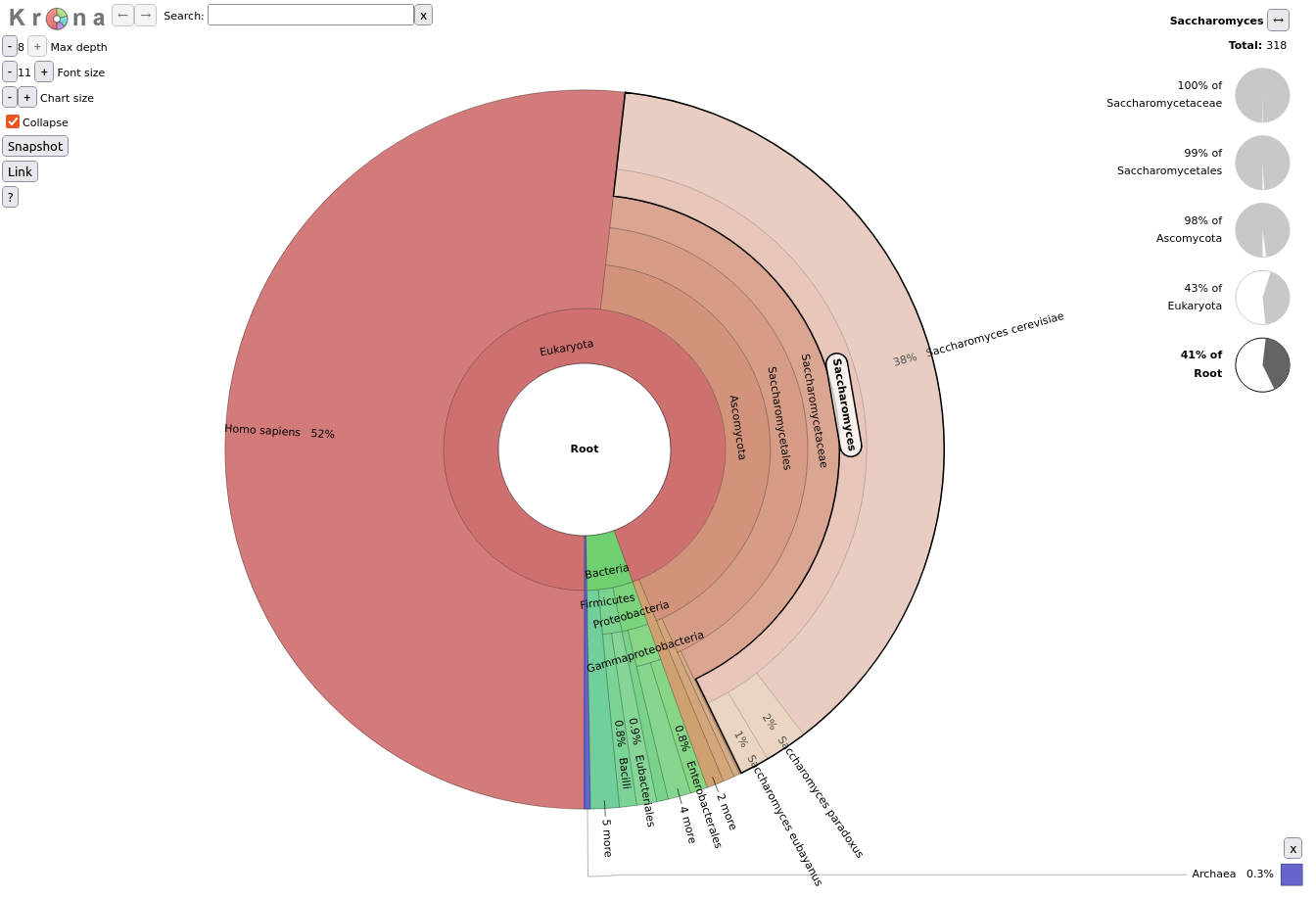
We can now run Krona. This tool creates an interactive report that allows hierarchical data (like taxonomy) to be explored with zooming, as multi-layered pie charts. With this tool, we can easily visualize the composition of a microbiome community.

Hands-on: Krona pie chart

1. Krona pie chart Tool: toolshed.g2.bx.psu.edu/repos/crs4/taxonomy_krona_chart/taxonomy_krona_chart/2.7.1 with the following parameters:
   • “What is the type of your input data”: Tabular
     • param-file “Input file”: output of Replace Text tool
2. Inspect the generated file

Let’s take a look at the result.

Question

1. What is the percentage of identified reads assigned to Homo sapiens? To Archaea?
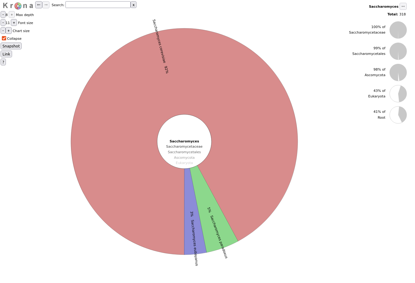
2. Click on Saccharomyces in the graph. What are the percentages of identified reads assigned to Saccharomyces for different levels?
3. Click a second time on Saccharomyces in the graph. What is the repartition between the different Saccharomyces species?

Solution

1. 52% of identified reads are assigned to Homo sapiens, and 0.3% of Archaea
2. Reads are assigned to Saccharomyces
   • 41% out of total identified reads (root)
   • 43% out of identified reads for Eukaryota domain
   • 98% out of identified reads for Ascomycota phylum
   • 99% out of identified reads for Saccharomycetales order
   • 100% out of identified reads for Saccharomycetaceae family

   

3. 92% of Saccharomyces reads are assigned to Saccharomyces cerevisiae, 5% to Saccharomyces paradoxus and 3% to Saccharomyces eubayanus,.

   

(Optional) Sharing your history

One of the most important features of Galaxy comes at the end of an analysis: sharing your histories with others so they can review them.

Tip: Sharing your History

Sharing your history allows others to import and access the datasets, parameters, and steps of your history.

1. Share via link
   • Open the History Options galaxy-gear menu (gear icon) at the top of your history panel
     • galaxy-toggle Make History accessible
     • A Share Link will appear that you give to others
   • Anybody who has this link can view and copy your history
2. Publish your history
   • galaxy-toggle Make History publicly available in Published Histories
   • Anybody on this Galaxy server will see your history listed under the Shared Data menu
3. Share only with another user.
   • Click the Share with a user button at the bottom
   • Enter an email address for the user you want to share with
   • Your history will be shared only with this user.
4. Finding histories others have shared with me
   • Click on User menu on the top bar
   • Select Histories shared with me
   • Here you will see all the histories others have shared with you directly

Note: If you want to make changes to your history without affecting the shared version, make a copy by going to galaxy-gear History options icon in your history and clicking Copy

Key points

• Data obtained by sequencing needs to be checked for quality and cleaned before further processing

• Yeast species but also contamination can be identified and visualized directly from the sequences using several bioinformatics tools

• With its graphical interface, Galaxy makes it easy to use the needed bioinformatics tools

• Beer microbiome is not just made of yeast and can be quite complex

Frequently Asked Questions

Useful literature

Further information, including links to documentation and original publications, regarding the tools, analysis techniques and the interpretation of results described in this tutorial can be found here.

References

1. Kurtzman, C. P., 1994 Molecular taxonomy of the yeasts. Yeast 10: 1727–1740.
2. Ondov, B. D., N. H. Bergman, and A. M. Phillippy, 2011 Interactive metagenomic visualization in a Web browser. BMC Bioinformatics 12: 10.1186/1471-2105-12-385
3. Wood, D. E., and S. L. Salzberg, 2014 Kraken: ultrafast metagenomic sequence classification using exact alignments. Genome Biology 15: R46. 10.1186/gb-2014-15-3-r46
4. Wick, R., 2017 Porechop. GitHub. https://github.com/rrwick/Porechop
5. Chen, S., Y. Zhou, Y. Chen, and J. Gu, 2018 fastp: an ultra-fast all-in-one FASTQ preprocessor. 10.1101/274100
6. Sampaio, J. P., 2018 Microbe profile: Saccharomyces eubayanus, the missing link to lager beer yeasts. Microbiology 164: 1069.
7. Wood, D. E., J. Lu, and B. Langmead, 2019 Improved metagenomic analysis with Kraken 2. Genome biology 20: 1–13.
8. Delahaye, C., and J. Nicolas, 2021 Sequencing DNA with nanopores: Troubles and biases. PLoS One 16: e0257521.

Feedback

Did you use this material as an instructor? Feel free to give us feedback on how it went.
Did you use this material as a learner or student? Click the form below to leave feedback.

Citing this Tutorial

1. Polina Polunina, Siyu Chen, Bérénice Batut, Teresa Müller, Identification of the micro-organisms in a beer using Nanopore sequencing (Galaxy Training Materials). https://training.galaxyproject.org/training-material/topics/metagenomics/tutorials/beer-data-analysis/tutorial.html Online; accessed TODAY
2. Batut et al., 2018 Community-Driven Data Analysis Training for Biology Cell Systems 10.1016/j.cels.2018.05.012

BibTeX

@misc{metagenomics-beer-data-analysis,
author = "Polina Polunina and Siyu Chen and Bérénice Batut and Teresa Müller",
title = "Identification of the micro-organisms in a beer using Nanopore sequencing (Galaxy Training Materials)",
year = "",
month = "",
day = ""
url = "\url{https://training.galaxyproject.org/training-material/topics/metagenomics/tutorials/beer-data-analysis/tutorial.html}",
note = "[Online; accessed TODAY]"
}
@article{Batut_2018,
    doi = {10.1016/j.cels.2018.05.012},
    url = {https://doi.org/10.1016%2Fj.cels.2018.05.012},
    year = 2018,
    month = {jun},
    publisher = {Elsevier {BV}},
    volume = {6},
    number = {6},
    pages = {752--758.e1},
    author = {B{\'{e}}r{\'{e}}nice Batut and Saskia Hiltemann and Andrea Bagnacani and Dannon Baker and Vivek Bhardwaj and Clemens Blank and Anthony Bretaudeau and Loraine Brillet-Gu{\'{e}}guen and Martin {\v{C}}ech and John Chilton and Dave Clements and Olivia Doppelt-Azeroual and Anika Erxleben and Mallory Ann Freeberg and Simon Gladman and Youri Hoogstrate and Hans-Rudolf Hotz and Torsten Houwaart and Pratik Jagtap and Delphine Larivi{\`{e}}re and Gildas Le Corguill{\'{e}} and Thomas Manke and Fabien Mareuil and Fidel Ram{\'{\i}}rez and Devon Ryan and Florian Christoph Sigloch and Nicola Soranzo and Joachim Wolff and Pavankumar Videm and Markus Wolfien and Aisanjiang Wubuli and Dilmurat Yusuf and James Taylor and Rolf Backofen and Anton Nekrutenko and Björn Grüning},
    title = {Community-Driven Data Analysis Training for Biology},
    journal = {Cell Systems}
}