Introduction

Molecular dynamics simulations return highly complex data. The Cartesian positions of each atom of the system (thousands or even millions) are recorded at every time step of the trajectory; this may again be thousands to millions of steps in length. Therefore, some kind of further analysis is needed to extract useful information from the data.

In this tutorial, we illustrate some of the analytical tools able to investigate conformational changes by analysis of a typical short protein simulation, such as for CBH1.

There are other analysis tools available; you are encouraged to try these out too.

Agenda

In this tutorial, we will cover:

1. Introduction
2. Get data
3. Analysis with BIO3D
   1. RMSD
   2. RMSF
   3. PCA
   4. Workflow vs. individual tools
4. Further analysis
5. Conclusion

Get data

The data required can be generated by completing the NAMD simulation tutorial. Access it from your history. Alternatively, download the data from the Zenodo link provided.

Hands-on: Upload cellulose simulation trajectory

1. Create a new history

   Tip: Creating a new history

   Click the new-history icon at the top of the history panel.

   If the new-history is missing:

   1. Click on the galaxy-gear icon (History options) on the top of the history panel
   2. Select the option Create New from the menu

2. Import the files from Zenodo, or from your history, if you completed the previous NAMD simulation tutorial:

   https://zenodo.org/record/2537734/files/cbh1test.dcd
   https://zenodo.org/record/2537734/files/cbh1test.pdb
   

   Tip: Importing via links

   • Copy the link location

   • Open the Galaxy Upload Manager (galaxy-upload on the top-right of the tool panel)

   • Select Paste/Fetch Data

   • Paste the link into the text field

   • Press Start

   • Close the window

3. Rename the dcd file ‘CBH1 trajectory’ and rename the pdb file ‘CBH1 structure’

   Tip: Renaming a dataset

   • Click on the galaxy-pencil pencil icon for the dataset to edit its attributes
   • In the central panel, change the Name field
   • Click the Save button

Analysis with BIO3D

We’ll carry out some basic analysis by calculating RMSD, RMSF and PCA. The tools use the Bio3D package, developed by the Grant lab.

RMSD

RMSD, or root-mean-square deviation, is a standard measure of structural distance between coordinates. It measures the average distance between a group of atoms (e.g. backbone atoms of a protein). If we calculate RMSD between two sets of atomic coordinates - for example, two time points from the trajectory - the value is a measure of how much the protein conformation has changed. Wikipedia provides more information.

Hands-on: Calculate RMSD

RMSD Analysis Tool: toolshed.g2.bx.psu.edu/repos/chemteam/bio3d_rmsd/bio3d_rmsd/2.3.4 with the following parameters:

• param-file “dcd trajectory input”: Trajectory file
• param-file “pdb input”: Structure file
• “Select domains”: Calpha (calculate RMSD only for the C-alpha domain of the protein)

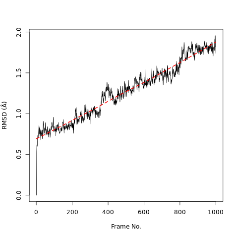
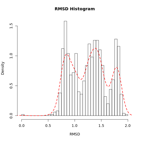
Question

What do the features in the RMSD plot tell us?

Solution

The increase in the RMSD plot with time shows the protein steadily deviates from its original conformation.

The three peaks visible in the histogram suggests the presence of three main conformations which are accessed during the trajectory.

RMSF

The root-mean-square fluctuation (RMSF) measures the average deviation of a particle (e.g. a protein residue) over time from a reference position (typically the time-averaged position of the particle). Thus, RMSF analyzes the portions of structure that are fluctuating from their mean structure the most (or least).

Hands-on: Calculate RMSF

1. RMSF Analysis Tool: toolshed.g2.bx.psu.edu/repos/chemteam/bio3d_rmsf/bio3d_rmsf/2.3.4 with the following parameters:
   • param-file “dcd trajectory input”: Trajectory file
   • param-file “pdb input”: Structure file
   • “Select domains”: Calpha (calculate RMSF only for the C-alpha domain of the protein)

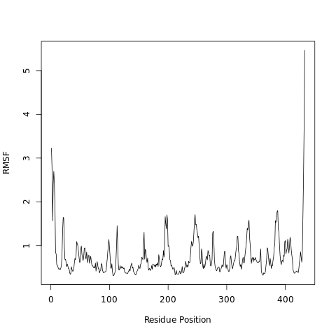
Question

What can we learn from the features in the RMSF plot?

Solution

Higher RMSF values most likely are loop regions with more conformational flexibility, where the structure is not as well defined.

This allows a link with experimental spectroscopic techniques which detect the secondary structure of a protein.

PCA

Principal component analysis (PCA) converts a set of correlated observations (movement of all atoms in protein) to a set of principal components which are linearly independent (or uncorrelated). Mathematically, it is a transformation of the data to a new coordinate system, in which the first coordinate represents the greatest variance, the second coordinate represents the second most variance, and so on.

You can read more about PCA on Wikipedia. In a nutshell, PCA takes a complex dataset with many variables and tries to distill the variables down to a few ‘principal components’ which still preserve most of the differences between the data.

In summary:

• The PCA tool tool will calculate and return a PCA to determine the relationship between statistically meaningful conformations (major global motions) sampled during the trajectory. THe tool returns several images of the PCA and the raw data in tab-separated format.
• The PCA visualization tool tool will carry out PCA and return a trajectory of the selected principle component. This trajectory is useful for visualisation and further investigating the interesting modes and changes that occur within a selected principle component.

Hands-on: Calculate PCA

1. PCA Tool: toolshed.g2.bx.psu.edu/repos/chemteam/bio3d_pca/bio3d_pca/2.3.4 with the following parameters:
   • param-file “dcd trajectory input”: Trajectory file
   • param-file “pdb input”: Structure file
   • “Use singular value decomposition (SVD) instead of default eigenvalue decomposition ?”: No
   • “Select domains”: Calpha
2. PCA visualization Tool: toolshed.g2.bx.psu.edu/repos/chemteam/bio3d_pca/bio3d_pca/2.3.4 with the following parameters:
   • param-file “dcd trajectory input”: Trajectory file
   • param-file “pdb input”: Structure file
   • “Use singular value decomposition (SVD) instead of default eigenvalue decomposition ?”: No
   • “Select domains”: Calpha
   • “Principal component id”: 1

PCA visualisation: This tool can generate small trajectories of the first three principal components. The .pdb of the .nc files can be visualized using a visualization software such as VMD.

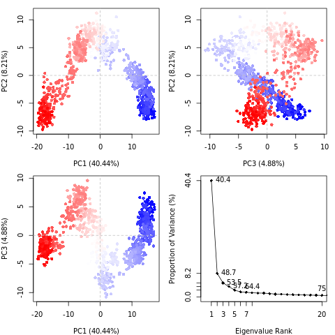
Question

What do the features in the RMSD plot tell us? Do the principal coordinates have a meaning?

Solution

Here, PCA shows the statistically meaningful conformations in the CBH1 trajectory. The principal motions within the trajectory and the vital motions needed for conformational changes can be identified. Two distinct groupings along the PC1 plane, indicating a non-periodic conformational change, are identified. The groupings along the PC2 and PC3 planes do not completely cluster separately, implying that these global motions are periodic. The PC1 is linked to an active site motion that limits the motion to a key glycosidic bond.

Workflow vs. individual tools

You can choose to use the tools one by one as described above, or alternatively combine into a single analysis using the workflow provided.

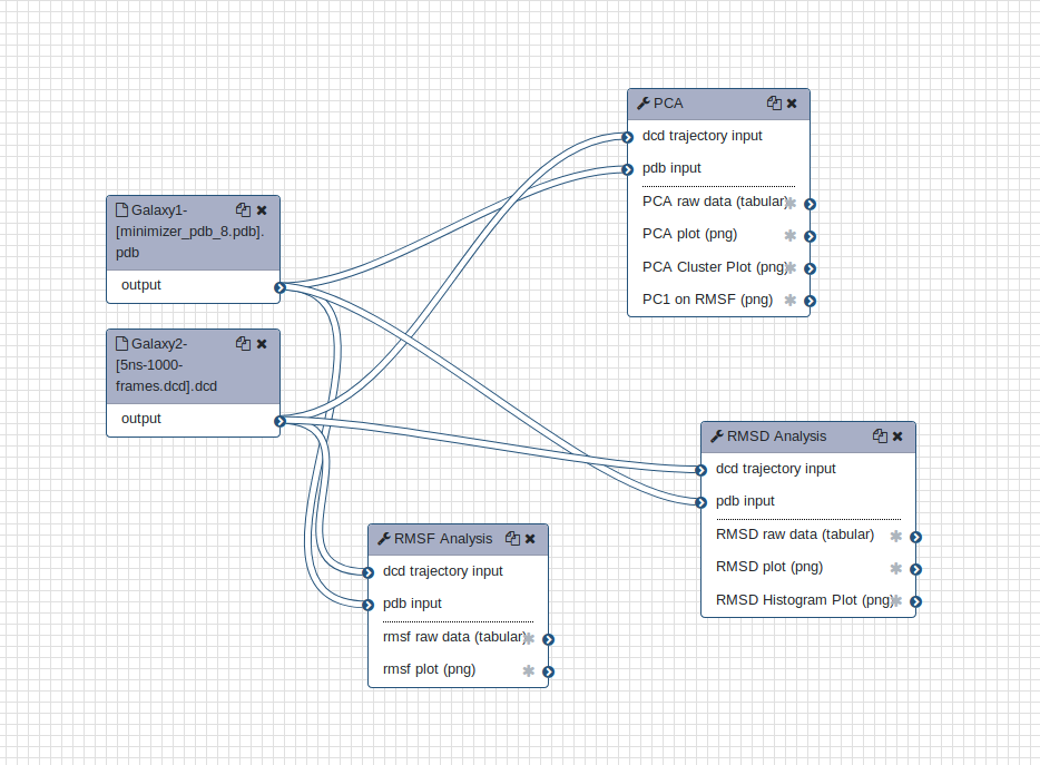
Hands-on: Upload a workflow

1. Click on ‘Workflow’ in the toolbar at the top of the main Galaxy page. In the upper right corner of the central pane, click the ‘Upload or import workflow’ icon.

2. Enter the ‘Archived workflow URL’ and click ‘Import workflow’.

   https://raw.githubusercontent.com/galaxyproject/training-material/master/topics/computational-chemistry/tutorials/analysis-md-simulations/workflows/main_workflow.ga
   

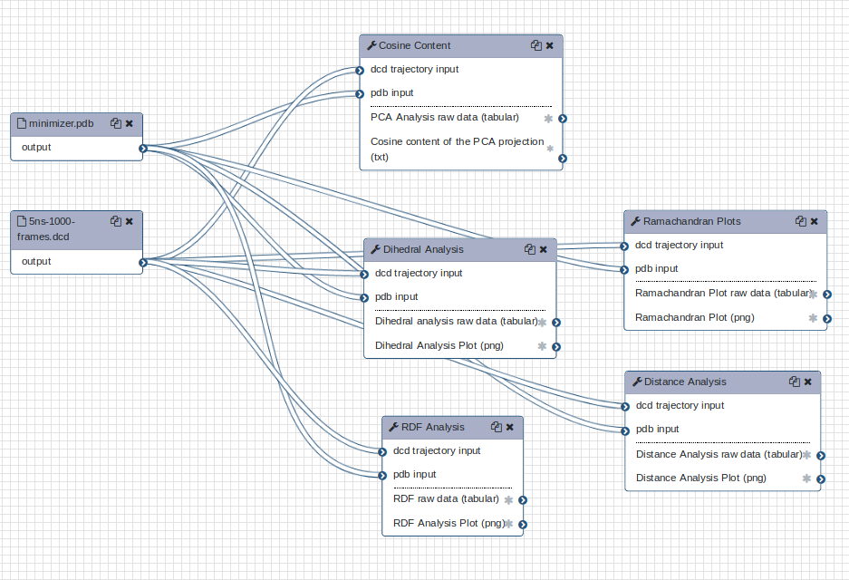
Further analysis

Further analyses are available; try out the MDAnalysis workflow, which includes a Ramachandran plot and various timeseries.

Conclusion

Key points

• Multiple analyses including timeseries, RMSD, PCA are available

• Analysis tools allow a further chemical understanding of the system

Frequently Asked Questions

Have questions about this tutorial? Check out the tutorial FAQ page or the FAQ page for the Computational chemistry topic to see if your question is listed there. If not, please ask your question on the GTN Gitter Channel or the Galaxy Help Forum

Useful literature

Further information, including links to documentation and original publications, regarding the tools, analysis techniques and the interpretation of results described in this tutorial can be found here.

Feedback

Did you use this material as an instructor? Feel free to give us feedback on how it went.
Did you use this material as a learner or student? Click the form below to leave feedback.

Citing this Tutorial

1. Christopher Barnett, Tharindu Senapathi, Simon Bray, Nadia Goué, Analysis of molecular dynamics simulations (Galaxy Training Materials). https://training.galaxyproject.org/training-material/topics/computational-chemistry/tutorials/analysis-md-simulations/tutorial.html Online; accessed TODAY
2. Batut et al., 2018 Community-Driven Data Analysis Training for Biology Cell Systems 10.1016/j.cels.2018.05.012

BibTeX

@misc{computational-chemistry-analysis-md-simulations,
author = "Christopher Barnett and Tharindu Senapathi and Simon Bray and Nadia Goué",
title = "Analysis of molecular dynamics simulations (Galaxy Training Materials)",
year = "",
month = "",
day = ""
url = "\url{https://training.galaxyproject.org/training-material/topics/computational-chemistry/tutorials/analysis-md-simulations/tutorial.html}",
note = "[Online; accessed TODAY]"
}
@article{Batut_2018,
    doi = {10.1016/j.cels.2018.05.012},
    url = {https://doi.org/10.1016%2Fj.cels.2018.05.012},
    year = 2018,
    month = {jun},
    publisher = {Elsevier {BV}},
    volume = {6},
    number = {6},
    pages = {752--758.e1},
    author = {B{\'{e}}r{\'{e}}nice Batut and Saskia Hiltemann and Andrea Bagnacani and Dannon Baker and Vivek Bhardwaj and Clemens Blank and Anthony Bretaudeau and Loraine Brillet-Gu{\'{e}}guen and Martin {\v{C}}ech and John Chilton and Dave Clements and Olivia Doppelt-Azeroual and Anika Erxleben and Mallory Ann Freeberg and Simon Gladman and Youri Hoogstrate and Hans-Rudolf Hotz and Torsten Houwaart and Pratik Jagtap and Delphine Larivi{\`{e}}re and Gildas Le Corguill{\'{e}} and Thomas Manke and Fabien Mareuil and Fidel Ram{\'{\i}}rez and Devon Ryan and Florian Christoph Sigloch and Nicola Soranzo and Joachim Wolff and Pavankumar Videm and Markus Wolfien and Aisanjiang Wubuli and Dilmurat Yusuf and James Taylor and Rolf Backofen and Anton Nekrutenko and Björn Grüning},
    title = {Community-Driven Data Analysis Training for Biology},
    journal = {Cell Systems}
}
                   

Congratulations on successfully completing this tutorial!

Do you want to extend your knowledge? Follow one of our recommended follow-up trainings:

• Computational chemistry
  • Analysis of molecular dynamics simulations: tutorial hands-on