Advances in sequencing technologies over the last few decades have revolutionized the field of genomics, allowing for a reduction in both the time and resources required to de novo genome assembly. Until recently, second-generation sequencing technologies (also known as Next Generation Sequencing or NGS) allowed to produce highly accurate but short (up to 800bp) reads, whose extension was not long enough to cope with the difficulties associated with repetitive regions. Today, so-called third-generation sequencing (TGS) technologies, usually known as single-molecule real-time (SMRT) sequencing, have become dominant in de novo assembly of large genomes. TGS can use native DNA without amplification, reducing sequencing error and bias (Hon et al. 2020, Giani et al. 2020). Very recently, Pacific Biosciences introduced High-Fidelity (HiFi) sequencing, which produces reads 10-25 kpb in length with a minimum accuracy of 99% (Q20). In this tutorial you will use HiFi reads in combination with data from additional sequencing technologies to generate a high-quality genome assembly.
Deciphering the structural organization of complex vertebrate genomes is currently one of the largest challenges in genomics (Frenkel et al. 2012). Despite the significant progress made in recent years, a key question remains: what combination of data and tools can produce the highest quality assembly? In order to adequately answer this question, it is necessary to analyse two of the main factors that determine the difficulty of genome assembly processes: repetitive content and heterozygosity.
Repetitive elements can be grouped into two categories: interspersed repeats, such as transposable elements (TE) that occur at multiple loci throughout the genome, and tandem repeats (TR) that occur at a single locus (Tørresen et al. 2019). Repetitive elements are an important component of eukaryotic genomes, constituting over a third of the genome in the case of mammals (Sotero-Caio et al. 2017, Chalopin et al. 2015). In the case of tandem repeats, various estimates suggest that they are present in at least one third of human protein sequences (Marcotte et al. 1999). TE content is among the main factors contributing to the lack of continuity in the reconstruction of genomes, especially in the case of large ones, as TE content is highly correlated with genome size (Sotero-Caio et al. 2017). On the other hand, TR usually lead to local genome assembly collapse, especially when their length is close to that of the reads (Tørresen et al. 2019).
Heterozygosity is also an important factor in genome assembly. Haplotype phasing, that is, the identification of alleles that are co-located on the same chromosome, has become a fundamental problem in heterozygous and polyploid genome assemblies (Zhang et al. 2020). When no reference sequence is available, the state-of-the-art strategy consists of constructing a string graph with vertices representing reads and edges representing consistent overlaps. In this kind of graph, after transitive reduction, heterozygous alleles in the string graph are represented by bubbles. When combined with Hi-C data, this approach allows complete diploid reconstruction (Angel et al. 2018, Zhang et al. 2020, Dida and Yi 2021).
The G10K consortium launched the Vertebrate Genomes Project (VGP), whose goal is generating high-quality, near-error-free, gap-free, chromosome-level, haplotype-phased, annotated reference genome assemblies for every vertebrate species (Rhie et al. 2021). This tutorial will guide you step by step to assemble a high-quality genome using the VGP assembly pipeline.
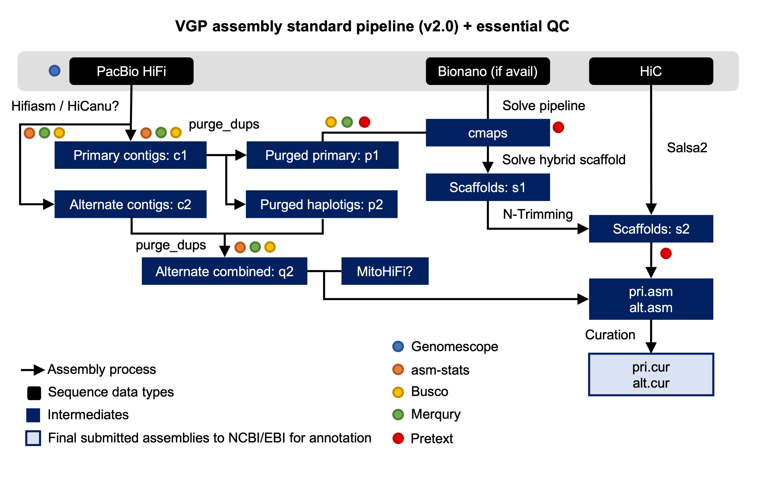
This training is an adaptation of the VGP assembly pipeline 2.0 (fig. 1).
Figure 1: VPG Pipeline 2.0. The pipeline starts with assembly of the HiFi reads into contigs, yielding the primary and alternate assemblies. Then, duplicated and erroneously assigned contigs will be removed by using purge_dups. Finally, Bionano optical maps and HiC data are used to generate a scaffolded primary assembly.
With the aim of making it easier to understand, the training has been organized into four main sections: genome profile analysis, HiFi phased assembly with hifiasm, post-assembly processing and hybrid scaffolding.
Get data
In order to reduce computation time, we will assemble samples from the yeast Saccharomyces cerevisiae S288C, a widely used laboratory strain isolated in the 1950s by Robert Mortimer. Using S. cerevisae, one of the most intensively studied eukaryotic model organisms, has the additional advantage of allowing us to evaluate the final result of our assembly with great precision. For this tutorial, we generated a set of synthetic HiFi reads corresponding to a theoretical diploid genome.
The synthetic HiFi reads were generated by using the S288C assembly as reference genome. With this objective we used HIsim, a HiFi shotgun simulator. The commands used are detailed below:
The selected mutation rate was 2%. Note that HIsim generates the synthetic reads in FASTA format. This is perfectly fine for illustrating the workflow, but you should be aware that usually you will work with HiFi reads in FASTQ format.
The first step is to get the datasets from Zenodo. The VGP assembly pipeline uses data generated by a variety of technologies, including PacBio HiFi reads, Bionano optical maps, and Hi-C chromatin interaction maps.
Copy the tabular data, paste it into the textbox and press Build
dataset_01    https://zenodo.org/record/6098306/files/HiFi_synthetic_50x_01.fasta?download=1  fasta    HiFi  HiFi_collection
dataset_02    https://zenodo.org/record/6098306/files/HiFi_synthetic_50x_02.fasta?download=1  fasta    HiFi  HiFi_collection
dataset_03    https://zenodo.org/record/6098306/files/HiFi_synthetic_50x_03.fasta?download=1  fasta    HiFi  HiFi_collection
From Rules menu select Add / Modify Column Definitions
Click Add Definition button and select List Identifier(s): column A
Click Add Definition button and select URL: column B
Click Add Definition button and select Type: column C
Click Add Definition button and select Group Tag: column D
Click Add Definition button and select Collection Name: column E
Click Apply and press Upload
HiFi reads preprocessing with Cutadapt
Adapter trimming usually means trimming the adapter sequence off the ends of reads, which is where the adapter sequence is usually located in NGS reads. However, due to the nature of SMRT sequencing technology, adapters do not have a specific, predictable location in HiFi reads. Additionally, the reads containing adapter sequence could be of generally lower quality compared to the rest of the reads. Thus, we will use Cutadapt not to trim, but to remove the entire read if a read is found to have an adapter inside of it.
Comment: Background on PacBio HiFi reads
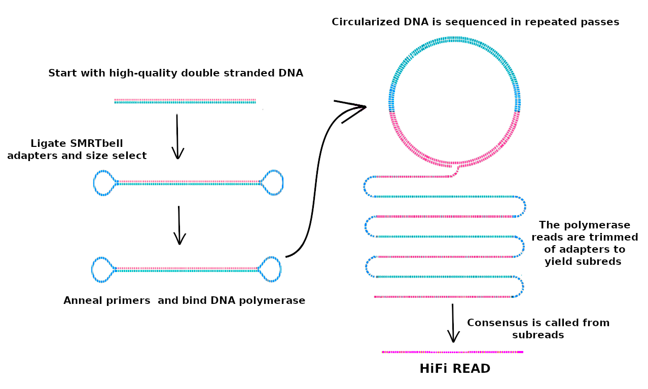
PacBio HiFi reads rely on the Single Molecule Real-Time (SMRT) sequencing technology. SMRT is based on real-time imaging of fluorescently tagged nucleotides as they are added to a newly synthesized DNA strand. HiFi further combine multiple subreads from the same circular template to produce one highly accurate consensus sequence (fig. 2).
Figure 2: HiFi reads are produced by calling consensus from subreads generated by multiple passes of the enzyme around a circularized template. This results in a HiFi read that is both long and accurate.
This technology allows to generate long-read sequencing data with read lengths in the range of 10-25 kb and minimum read consensus accuracy greater than 99% (Q20).
Hands-on: Primer removal with Cutadapt
CutadaptTool: toolshed.g2.bx.psu.edu/repos/lparsons/cutadapt/cutadapt/3.4 with the following parameters:
“Single-end or Paired-end reads?”: Single-end
param-collection“FASTQ/A file”: HiFi_collection
In “Read 1 Options”:
In “5’ or 3’ (Anywhere) Adapters”:
param-repeat“Insert 5’ or 3’ (Anywhere) Adapters”
“Source”: Enter custom sequence
“Enter custom 5’ or 3’ adapter name”: First adapter
“Enter custom 5’ or 3’ adapter sequence”: ATCTCTCTCAACAACAACAACGGAGGAGGAGGAAAAGAGAGAGAT
param-repeat“Insert 5’ or 3’ (Anywhere) Adapters”
“Source”: Enter custom sequence
“Enter custom 5’ or 3’ adapter name”: Second adapter
“Enter custom 5’ or 3’ adapter sequence”: ATCTCTCTCTTTTCCTCCTCCTCCGTTGTTGTTGTTGAGAGAGAT
In “Adapter Options”:
“Maximum error rate”: 0.1
“Minimum overlap length”: 35
“Look for adapters in the reverse complement”: Yes
In “Filter Options”:
“Discard Trimmed Reads”: Yes
Click on param-collectionDataset collection in front of the input parameter you want to supply the collection to.
Select the collection you want to use from the list
Rename the output file as HiFi_collection (trim).
Click on the galaxy-pencilpencil icon for the dataset to edit its attributes
Before starting a de novo genome assembly project, it is useful to collect metrics on the properties of the genome under consideration, such as the expected genome size. Traditionally, DNA flow cytometry was considered the golden standard for estimating the genome size. Nowadays, experimental methods have been replaced by computational approaches (Wang et al. 2020). One of the widely used genome profiling methods is based on the analysis of k-mer frequencies. It allows one to provide information not only about the genomic complexity, such as the genome size and levels of heterozygosity and repeat content, but also about the data quality.
Comment: K-mer size, sequencing coverage and genome size
K-mers are unique substrings of length k contained within a DNA sequence. For example, the DNA sequence TCGATCACA can be decomposed into five unique k-mers that have five bases long: TCGAT, CGATC, GATCA, ATCAC and TCACA. A sequence of length L will have L-k+1 k-mers. On the other hand, the number of possible k-mers can be calculated as nk, where n is the number of possible monomers and k is the k-mer size.
Bases
K-mer size
Total possible k-mers
4
1
4
4
2
16
4
3
64
4
…
…
4
10
1.048.576
Thus, the k-mer size is a key parameter, which must be large enough to map uniquely to the genome, but not too large, since it can lead to wasting computational resources. In the case of the human genome, k-mers of 31 bases in length lead to 96.96% of unique k-mers.
Each unique k-mer can be assigned a value for coverage based on the number of times it occurs in a sequence, whose distribution will approximate a Poisson distribution, with the peak corresponding to the average genome sequencing depth. From the genome coverage, the genome size can be easily computed.
Generation of k-mer spectra with Meryl
Meryl will allow us to generate the k-mer profile by decomposing the sequencing data into k-length substrings, counting the occurrence of each k-mer and determining its frequency. The original version of Meryl was developed for the Celera Assembler. The current Meryl version comprises three main modules: one for generating k-mer databases, one for filtering and combining databases, and one for searching databases. K-mers are stored in lexicographical order in the database, similar to words in a dictionary (Rhie et al. 2020).
Comment: k-mer size estimation
Given an estimated genome size (G) and a tolerable collision rate (p), an appropriate k can be computed as k = log4 (G(1 − p)/p).
Hands-on: Generate k-mers count distribution
Run MerylTool: toolshed.g2.bx.psu.edu/repos/iuc/meryl/meryl/1.3+galaxy2 with the following parameters:
“Operation type selector”: Count operations
“Count operations”: Count: count the occurrences of canonical k-mers
We used 32 as k-mer size, as this length has demonstrated to be sufficiently long that most k-mers are not repetitive and is short enough to be more robust to sequencing errors. For very large (haploid size > 10 Gb) and/or very repetitive genomes, larger k-mer length is recommended to increase the number of unique k-mers.
Rename it Collection meryldb
Run MerylTool: toolshed.g2.bx.psu.edu/repos/iuc/meryl/meryl/1.3+galaxy1 again with the following parameters:
“Operation type selector”: Operations on sets of k-mers
“Operations on sets of k-mers”: Union-sum: return k-mers that occur in any input, set the count to the sum of the counts
param-file“Input meryldb”: Collection meryldb
Rename it as Merged meryldb
Run MerylTool: toolshed.g2.bx.psu.edu/repos/iuc/meryl/meryl/1.3+galaxy0 for the third time with the following parameters:
“Operation type selector”: Generate histogram dataset
param-file“Input meryldb”: Merged meryldb
Finally, rename it as Meryldb histogram.
Genome profiling with GenomeScope2
The next step is to infer the genome properties from the k-mer histogram generated by Meryl, for which we will use GenomeScope2. Genomescope2 relies on a nonlinear least-squares optimization to fit a mixture of negative binomial distributions, generating estimated values for genome size, repetitiveness, and heterozygosity rates (Ranallo-Benavidez et al. 2020).
Hands-on: Estimate genome properties
GenomeScopeTool: toolshed.g2.bx.psu.edu/repos/iuc/genomescope/genomescope/2.0 with the following parameters:
“k-mer length used to calculate k-mer spectra”: 32
In “Output options”: mark Summary of the analysis
In “Advanced options”:
“Create testing.tsv file with model parameters”: Yes
Genomescope will generate six outputs:
Plots
Linear plot: k-mer spectra and fitted models: frequency (y-axis) versus coverage.
Log plot: logarithmic transformation of the previous plot.
Transformed linear plot: k-mer spectra and fitted models: frequency times coverage (y-axis) versus coverage (x-axis). This transformation increases the heights of higher-order peaks, overcoming the effect of high heterozygosity.
Transformed log plot: logarithmic transformation of the previous plot.
Model: this file includes a detailed report about the model fitting.
Summary: it includes the properties inferred from the model, such as genome haploid length and the percentage of heterozygosity.
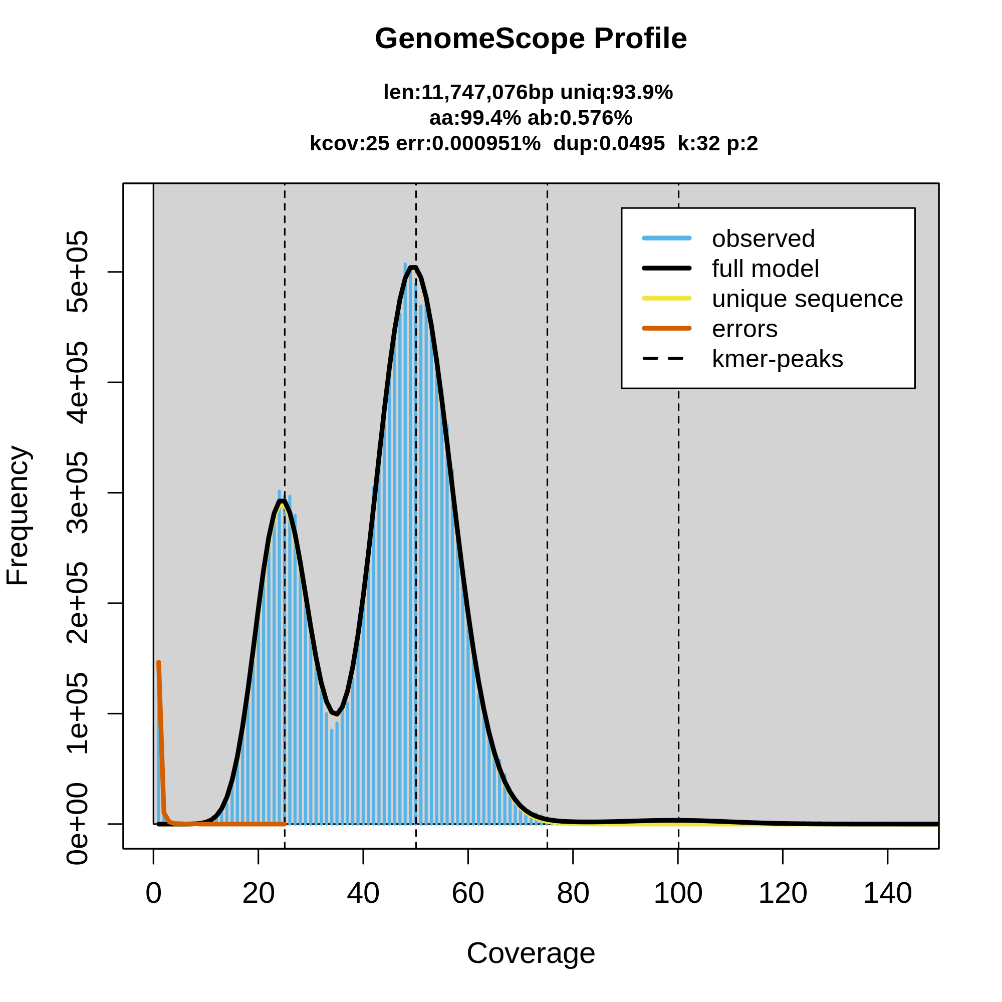
Now, let’s analyze the k-mer profiles, fitted models and estimated parameters (fig. 3).
Figure 3: GenomeScope2 32-mer profile. The first peak located at coverage 32x corresponds to the heterozygous peak. The second peak at coverage 50x, corresponds to the homozygous peak. Estimate of the heterozygous portion is 0.576%. The plot also includes informatin about the inferred total genome length (len), genome unique length percent (uniq), overall heterozygosity rate (het), mean k-mer coverage for heterozygous bases (kcov), read error rate (err), average rate of read duplications (dup) and k-mer size (k).
This distribution is the result of the Poisson process underlying the generation of sequencing reads. As we can see, the k-mer profile follows a bimodal distribution, indicative of a diploid genome. The distribution is consistent with the theoretical diploid model (model fit > 93%). Low frequency k-mers are the result of sequencing errors. GenomeScope2 estimated a haploid genome size is around 11.7 Mb, a value reasonably close to Saccharomyces genome size. Additionally, it revealed that the variation across the genomic sequences is 0.576%.
Before proceeding to the next section, we need to carry out some text manipulation operations on the output generated by GenomeScope2 to make it compatible with downstream tools. The goal is to extract some parameters which at a later stage will be used by purge_dups.
The first relevant parameter is the estimated genome size.
Hands-on: Get estimated genome size
Replace parts of textTool: toolshed.g2.bx.psu.edu/repos/bgruening/text_processing/tp_find_and_replace/1.1.3 with the following parameters:
param-file“File to process”: summary (output of GenomeScopetool)
“Find pattern”: bp
“Replace with”: leave this field empty (as it is)
“Replace all occurrences of the pattern”: Yes
“Find and Replace text in”: entire line
Replace parts of textTool: toolshed.g2.bx.psu.edu/repos/bgruening/text_processing/tp_find_and_replace/1.1.3 with the following parameters:
param-file“File to process”: output file of Replacetool
“Find pattern”: ,
“Replace with”: leave this field empty (as it is)
“Replace all occurrences of the pattern”: Yes
“Find and Replace text in”: entire line
Search in textfiles (grep)Tool: toolshed.g2.bx.psu.edu/repos/bgruening/text_processing/tp_grep_tool/1.1.1 with the following parameters:
param-file“Select lines from”: output file of the previous step.
“Type of regex”: Basic
“Regular Expression”: Haploid
Convert delimiters to TABTool: Convert characters1 with the following parameters:
param-file“in Dataset”: output of Search in textfilestool
Advanced CutTool: toolshed.g2.bx.psu.edu/repos/bgruening/text_processing/tp_cut_tool/1.1.0 with the following parameters:
param-file“File to cut”: output of Convert delimiters to TABtool
“Cut by”: fields
“List of Fields”: Column: 5
Rename the output as Estimated genome size.
Question
What is the estimated genome size?
The estimated genome size is 11.747.076 bp.
Now let’s parse the upper bound for the read depth estimation parameter. This parameter will be used later by purge_dups as high read depth cutoff to identify junk contigs.
Hands-on: Get maximum read depth
Compute an expression on every rowTool: toolshed.g2.bx.psu.edu/repos/devteam/column_maker/Add_a_column1/1.6 with the following parameters:
“Add expression”: 1.5*c3
param-file“as a new column to”: model_params (output of GenomeScopetool)
“Round result?”: Yes
“Input has a header line with column names?”: No
Compute an expression on every rowTool: toolshed.g2.bx.psu.edu/repos/devteam/column_maker/Add_a_column1/1.6 with the following parameters:
“Add expression”: 3*c7
param-file“as a new column to”: output of the previous step.
“Round result?”: Yes
“Input has a header line with column names?”: No
Rename it as Parsing temporal output
Advanced CutTool: toolshed.g2.bx.psu.edu/repos/bgruening/text_processing/tp_cut_tool/1.1.0 with the following parameters:
param-file“File to cut”: Parsing temporal output
“Cut by”: fields
“List of Fields”: Column 8
Rename the output as Maximum depth
Question
What is the estimated maximum depth?
What does this parameter represent?
The estimated maximum depth is 114 reads.
The maximum depth indicates the maximum number of sequencing reads that align to specific positions in the genome.
Finally, let’s parse the transition between haploid and diploid coverage depths parameter. This will be used as threshold to discriminate between haploid and diploid depths.
Hands-on: Get transition parameter
Advanced CutTool: toolshed.g2.bx.psu.edu/repos/bgruening/text_processing/tp_cut_tool/1.1.0 with the following parameters:
Once we have finished the genome profiling stage, we can start the genome assembly with hifiasm, a fast open-source de novo assembler specifically developed for PacBio HiFi reads.
Genome assembly with hifiasm
One of the key advantages of hifiasm is that it allows us to resolve near-identical, but not exactly identical sequences, such as repeats and segmental duplications (Cheng et al. 2021).
Comment: Hifiasm algorithm details
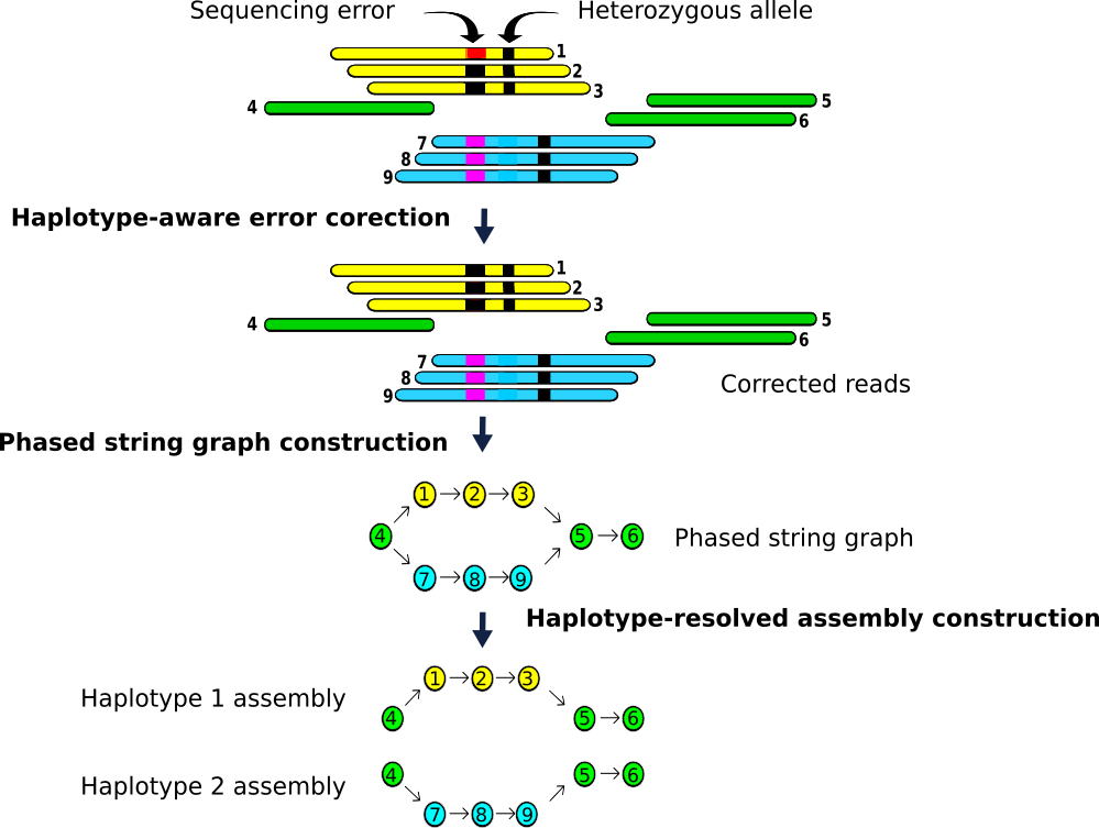
By default hifiasm performs three rounds of haplotype-aware error correction to correct sequence errors but keeping heterozygous alleles. A position on the target read to be corrected is considered informative if there are two different nucleotides at that position in the alignment, and each allele is supported by at least three reads.
Figure 4: Hifiasm algorithm overview. Orange and blue bars represent the reads with heterozygous alleles carrying local phasing information, while green bars come from the homozygous regions without any heterozygous alleles.
Then, hifiasm builds a phased assembly string graph with local phasing information from the corrected reads. Only the reads coming from the same haplotype are connected in the phased assembly graph. After transitive reduction, a pair of heterozygous alleles is represented by a bubble in the string graph. If there is no additional data, hifiasm arbitrarily selects one side of each bubble and outputs a primary assembly. In the case of a heterozygous genome, the primary assembly generated at this step may still retain haplotigs from the alternate allele.
Hands-on: Phased assembly with hifiasm
HifiasmTool: toolshed.g2.bx.psu.edu/repos/bgruening/hifiasm/hifiasm/0.14+galaxy0 with the following parameters:
“Assembly mode”: Standard
param-file“Input reads”: HiFi_collection (trim) (output of Cutadapttool)
After the tool has finished running rename its outputs as follows:
Rename the Hi-C hap1 balanced contig graph as Primary contigs graph and add a #primary tag
Rename the Hi-C hap2 balanced contig graph as Alternate contigs graph and add a #alternate tag
Hifiasm generates four outputs in Graphical Fragment Assembly (GFA) format; this format is designed to represent genome variation, splice graphs in genes, and even overlaps between reads.
We have obtained the fully phased contig graphs of the primary and alternate haplotypes, but the output format of hifiasm must be converted to FASTA format for the subsequent steps.
Hands-on: convert GFA to FASTA
GFA to FASTATool: toolshed.g2.bx.psu.edu/repos/iuc/gfa_to_fa/gfa_to_fa/0.1.2 with the following parameters:
param-files“Input GFA file”: select Primary contigs graph and the Alternate contigs graph datasets
Click on param-filesMultiple datasets
Select several files by keeping the Ctrl (or COMMAND) key pressed and clicking on the files of interest
Rename the outputs as Primary contigs FASTA and Alternate contigs FASTA
Initial assembly evaluation
The VGP assembly pipeline contains several built-in QC steps, including QUAST, BUSCO (Benchmarking Universal Single-Copy Orthologs), Merqury, and Pretext. QUAST will generate summary statistics, BUSCO will search for universal single-copy ortholog genes, Merqury will evaluate assembly copy-numbers using k-mers, and Pretext will be used to evaluate the assembly contiguity.
Comment: QUAST statistics
QUAST will provide us with the following statistics:
No. of contigs: The total number of contigs in the assembly.
Largest contig: The length of the largest contig in the assembly.
Total length: The total number of bases in the assembly.
Nx: The largest contig length, L, such that contigs of length >= L account for at least x% of the bases of the assembly.
NGx: The contig length such that using equal or longer length contigs produces x% of the length of the reference genome, rather than x% of the assembly length.
GC content: the percentage of nitrogenous bases which are either guanine or cytosine.
QUAST default pipeline utilizes Minimap2. Functional elements prediction modules include GeneMarkS, GeneMark-ES, GlimmerHMM, Barrnap, and BUSCO.
Hands-on: assembly evaluation with QUAST
QuastTool: toolshed.g2.bx.psu.edu/repos/iuc/quast/quast/5.0.2+galaxy1 with the following parameters:
“Use customized names for the input files?”: Yes, specify custom names
In “1. Contigs/scaffolds”:
param-file“Contigs/scaffolds file”: Primary contigs FASTA
“Name”: Primary assembly
Click in “Insert Contigs/scaffolds”
In “2. Contigs/scaffolds”:
param-file“Contigs/scaffolds file”: Alternate contigs FASTA
“Estimated reference genome size (in bp) for computing NGx statistics”: 11747076 (previously estimated)
“Type of organism”: Eukaryote: use of GeneMark-ES for gene finding, Barrnap for ribosomal RNA genes prediction, BUSCO for conserved orthologs finding (--eukaryote)
“Is genome large (>100Mpb)?”: No
Comment
Remember that for this training we are using S. cerevisiae, a reduced genome. In the case of assembling a vertebrate genome, you must select yes in the previous option.
Rename the HTML report as QUAST initial report
Let’s have a look at the HTML report generated by QUAST.
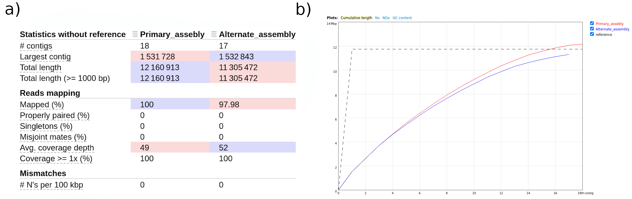
Figure 5: QUAST HTML report. Statistics of the primary and alternate assembly (a). Cumulative length plot. It shows the growth of contig lengths. On the x-axis, contigs are ordered from the largest to smallest. The y-axis gives the size of the x largest contigs in the assembly (b).
According to the report, both assemblies are quite similar; the primary assembly includes 18 contigs, whose cumulative length is around 12.1Mbp. On the other hand, the second alternate assembly includes 17 contigs, whose total lenght is 11.3Mbp. As we can see in the figure 5b, the alternate assembly is slighly smaller than the primary assembly.
Question
What is the longest contig in the primary assembly? And in the alternate one?
What is the N50 of the primary assembly?
Which percentage of reads mapped to each assembly?
The longest contig in the primary assembly is 1.531.728 bp, and 1.532.843 bp in the alternate assembly.
The N50 of the primary assembly is 813.039 bp.
According to the report, 100% of reads mapped to both the primary assembly and 97.98% to the alternate assembly.
Next, we will use BUSCO, which will provide quantitative assessment of the completeness of a genome assembly in terms of expected gene content. It relies on the analysis of genes that should be present only once in a complete assembly or gene set, while allowing for rare gene duplications or losses (Simão et al. 2015).
Hands-on: assessing assembly completeness with BUSCO
BuscoTool: toolshed.g2.bx.psu.edu/repos/iuc/busco/busco/5.0.0+galaxy0 with the following parameters:
param-files“Sequences to analyze”: Primary contigs FASTA and Alternate contigs FASTA
“Mode”: Genome assemblies (DNA)
“Use Augustus instead of Metaeuk”: Use Metaeuk
“Auto-detect or select lineage?”: Select lineage
“Lineage”: Saccharomycetes
“Which outputs should be generated”: short summary text
Comment
Remember to modify the lineage option if you are working with vertebrate genomes.
Rename the summary as BUSCO initial report primary and BUSCO initial report alternate.
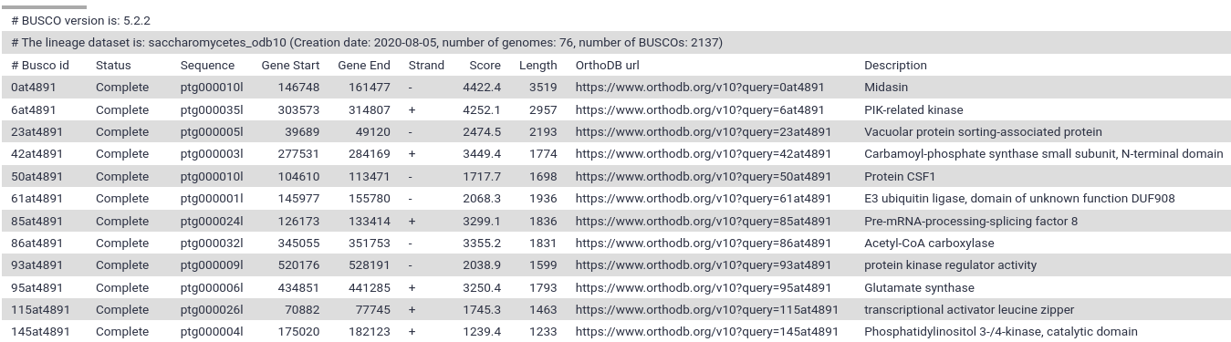
BUSCO generates two outputs by default: a complete report for each BUSCO gene (fig. 6), and a short summary.
Figure 6: BUSCO full table. It contains the complete results in a tabular format with scores and lengths of BUSCO matches, and coordinates.
As we can see in the figure, the detailed report includes valuable information, such as the status of the gene identified in the input sequence, its position (start/end coordinates and strand), the BUSCO score, the gene length and a keyword description.
Question
How many complete BUSCO genes have been identified in the primary assembly? You can find that information in the short summary.
How many BUSCOs genes are absent?
According to the report, our assembly contains the complete sequence of 2046 complete BUSCO genes (95.7%).
29 BUSCO genes are missing.
Despite BUSCO being robust for species that have been widely studied, it can be inaccurate when the newly assembled genome belongs to a taxonomic group that is not well represented in OrthoDB. Merqury provides a complementary approach for assessing genome assembly quality metrics in a reference-free manner via k-mer copy number analysis.
Hands-on: k-mer based evaluation with Merqury
MerquryTool: toolshed.g2.bx.psu.edu/repos/iuc/merqury/merqury/1.3 with the following parameters:
“Evaluation mode”: Default mode
param-file“k-mer counts database”: Merged meryldb
“Number of assemblies”: `Two assemblies
param-file“First genome assembly”: Primary contigs FASTA
param-file“Second genome assembly”: Alternate contigs FASTA
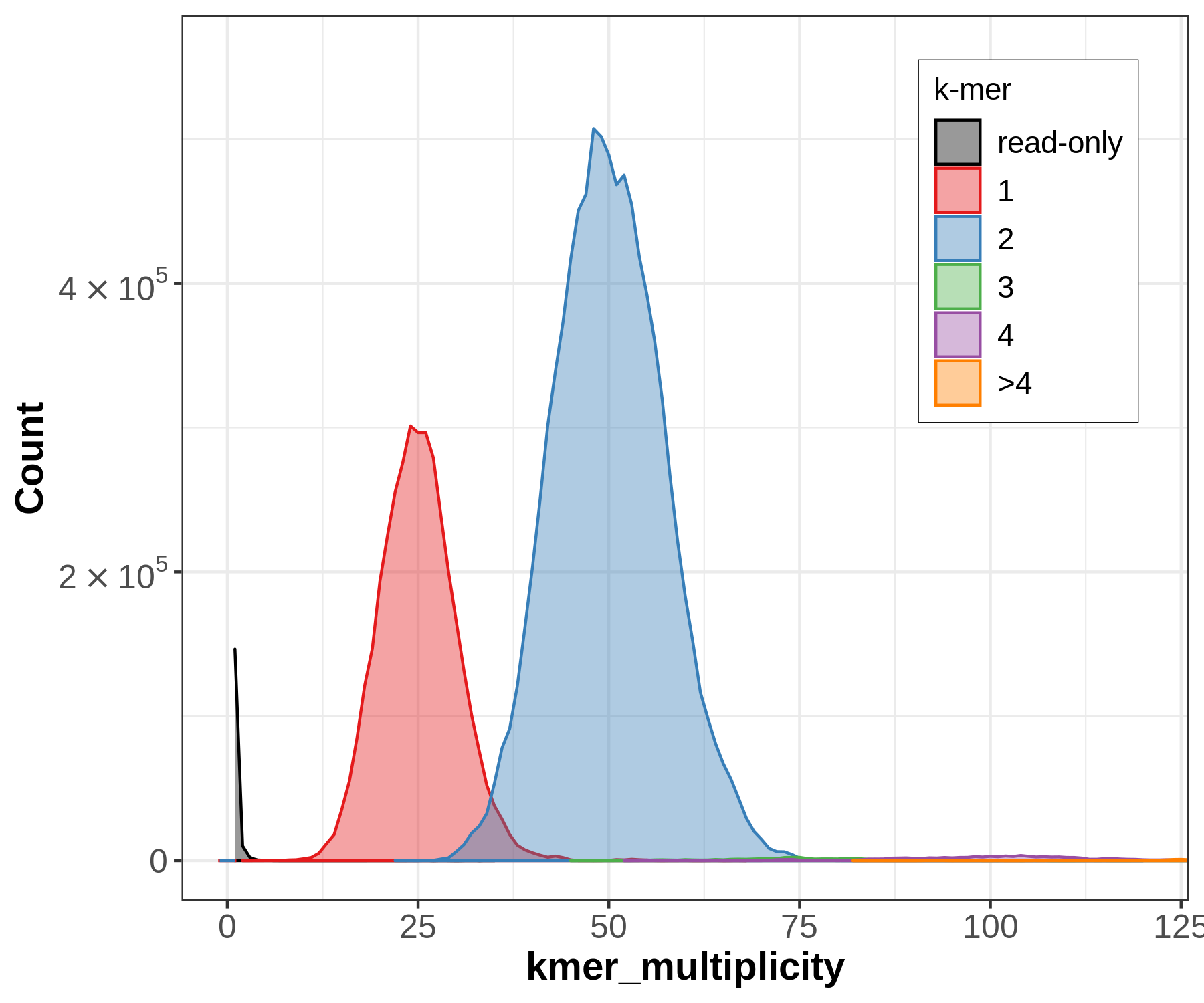
By default, Merqury generates three collections as output: stats, plots and QV stats. The “stats” collection contains the completeness statistics, while the “QV stats” collection contains the quality value statistics. Let’s have a look at the primary assembly copy number (CN) spectrum plot, known as the spectra-cn plot (fig. 7).
Figure 7: Merqury CN plot. This plot tracks the multiplicity of each k-mer found in the Hi-Fi read set and colors it by the number of times it is found in a given assembly. Merqury connects the midpoint of each histogram bin with a line, giving the illusion of a smooth curve.
The black region in the left side corresponds to k-mers found only in the read set; it is usually indicative of sequencing error in the read set, although it can also be indicative of missing sequences in the assembly. The read area represents one-copy k-mers in the genome, while blue area represents two-copy k-mers originating from homozygous sequence or haplotype-specific duplications. From that figure we can state that the sequencing coverage is around 50x.
An ideal haploid representation would consist of one allelic copy of all heterozygous regions in the two haplomes, as well as all hemizygous regions from both haplomes (Guan et al. 2019). However, in highly heterozygous genomes, assembly algorithms are frequently not able to identify the highly divergent allelic sequences as belonging to the same region, resulting in the assembly of those regions as separate contigs. This can lead to issues in downstream analysis, such as scaffolding, gene annotation and read mapping in general (Small et al. 2007, Guan et al. 2019, Roach et al. 2018). In order to solve this problem, we are going to use purge_dups; this tool will allow us to identify and reassign allelic contigs.
Remove haplotypic duplication with purge_dups
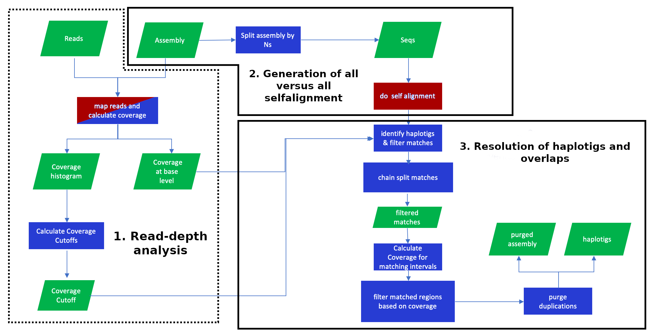
This stage consists of three substages: read-depth analysis, generation of all versus all self-alignment and resolution of haplotigs and overlaps (fig. 8).
Figure 8: Purge_dups pipeline. Adapted from github.com/dfguan/purge_dups. Purge_dups is integrated in a multi-step pipeline consisting in three main substages. Red indicates the steps which require to use Minimap2.
Read-depth analysis
Initially, we need to collapse our HiFi trimmed reads collection into a single dataset.
Hands-on: Collapse the collection
Collapse CollectionTool: toolshed.g2.bx.psu.edu/repos/nml/collapse_collections/collapse_dataset/4.2 with the following parameters:
param-collection“Collection of files to collapse into single dataset”:HiFi_collection (trim)
Rename the output as HiFi reads collapsed
Now, we will map the reads against the primary assembly by using Minimap2 (Li 2018), an alignment program designed to map long sequences.
Hands-on: Map the reads to contigs with Minimap2
Map with minimap2Tool: toolshed.g2.bx.psu.edu/repos/iuc/minimap2/minimap2/2.17+galaxy4 with the following parameters:
“Will you select a reference genome from your history or use a built-in index?”: Use a genome from history and build index
param-file“Use the following dataset as the reference sequence”: Primary contigs FASTA
“Select a profile of preset options”: Long assembly to reference mapping (-k19 -w19 -A1 -B19 -O39,81 -E3,1 -s200 -z200 --min-occ-floor=100). Typically, the alignment will not extend to regions with 5% or higher sequence divergence. Only use this preset if the average divergence is far below 5%. (asm5)
In “Set advanced output options”:
“Select an output format”: paf
Rename the output as Reads mapped to contigs
Finally, we will use the Reads mapped to contigs pairwise mapping format (PAF) file for calculating some statistics required in a later stage. In this step, purge_dups (listed as Purge overlaps in Galaxy tool panel) initially produces a read-depth histogram from base-level coverages. This information is used for estimating the coverage cutoffs, taking into account that collapsed haplotype contigs will lead to reads from both alleles mapping to those contigs, whereas if the alleles have assembled as separate contigs, then the reads will be split over the two contigs, resulting in half the read-depth (Roach et al. 2018).
Hands-on: Read-depth analisys
Purge overlapsTool: toolshed.g2.bx.psu.edu/repos/iuc/purge_dups/purge_dups/1.2.5+galaxy3 with the following parameters:
“Function mode”: Calculate coverage cutoff, base-level read depth and create read depth histogram for PacBio data (calcuts+pbcstats)
param-file“PAF input file”: Reads mapped to contigs
In “Calcuts options”:
“Transition between haploid and diploid”: 38
“Upper bound for read depth”: 114 (the previously estimated maximum depth)
“Ploidity”: Diploid
Rename the outputs as PBCSTAT base coverage primary, Histogram plot primary and Calcuts cutoff primary.
Purge overlaps (purge_dups) generates three outputs:
PBCSTAT base coverage: it contains the base-level coverage information.
Calcuts-cutoff: it includes the thresholds calculated by purge_dups.
Histogram plot.
Generation of all versus all self-alignment
Now, we will segment the draft assembly into contigs by cutting at blocks of Ns, and use minimap2 to generate an all by all self-alignment.
Hands-on: purge_dups pipeline
Purge overlapsTool: toolshed.g2.bx.psu.edu/repos/iuc/purge_dups/purge_dups/1.2.5+galaxy2 with the following parameters:
“Function mode”: split assembly FASTA file by 'N's (split_fa)
param-file“Assembly FASTA file”: Primary contigs FASTA
Rename the output as Split FASTA
Map with minimap2Tool: toolshed.g2.bx.psu.edu/repos/iuc/minimap2/minimap2/2.17+galaxy4 with the following parameters:
“Will you select a reference genome from your history or use a built-in index?”: Use a genome from history and build index
param-file“Use the following dataset as the reference sequence”: Split FASTA
“Single or Paired-end reads”: Single
param-file“Select fastq dataset”: Split FASTA
“Select a profile of preset options”: Construct a self-homology map - use the same genome as query and reference (-DP -k19 -w 19 -m200) (self-homology)
In “Set advanced output options”:
“Select an output format”: PAF
Rename the output as Self-homology map primary
Resolution of haplotigs and overlaps
During the final step of the purge_dups pipeline, it will use the self alignments and the cutoffs for identifying the haplotypic duplications.
In order to identify the haplotypic duplications, purge_dups uses the base-level coverage information to flag the contigs according the following criteria:
If more than 80% bases of a contig are above the high read depth cutoff or below the noise cutoff, it is discarded.
If more than 80% bases are in the diploid depth interval, it is labeled as a primary contig, otherwise it is considered further as a possible haplotig.
Contigs that were flagged for further analysis according to read-depth are then evaluated to attempt to identify synteny with its allelic companion contig. In this step, purge_dups uses the information contained in the self alignments:
If the alignment score is larger than the cutoff s (default 70), the contig is marked for reassignment as haplotig. Contigs marked for reassignment with a maximum match score greater than the cutoff m (default 200) are further flagged as repetitive regions.
Otherwise contigs are considered as a candidate primary contig.
Once all matches associated with haplotigs have been removed from the self-alignment set, purge_dups ties consistent matches between the remaining candidates to find collinear matches, filtering all the matches whose score is less than the minimum chaining score l.
Finally, purge_dups calculates the average coverage of the matching intervals for each overlap, and mark an unambiguous overlap as heterozygous when the average coverage on both contigs is less than the read-depth cutoff, removing the sequences corresponding to the matching interval in the shorter contig.
Hands-on: Resolution of haplotigs and overlaps
Purge overlapsTool: toolshed.g2.bx.psu.edu/repos/iuc/purge_dups/purge_dups/1.2.5+galaxy5 with the following parameters:
“Select the purge_dups function”: Purge haplotigs and overlaps for an assembly (purge_dups)
param-file“Base-level coverage file”: PBCSTAT base coverage primary
param-file“Cutoffs file”: calcuts cutoff primary
Rename the output as purge_dups BED
Purge overlapsTool: toolshed.g2.bx.psu.edu/repos/iuc/purge_dups/purge_dups/1.2.5+galaxy2 with the following parameters:
“Select the purge_dups function”: Obtain sequences after purging (get_seqs)
param-file“Assembly FASTA file”: Primary contigs FASTA
param-file“BED input file”: purge_dups BED (output of the previous step)
Rename the output get_seq purged sequences as Primary contigs purged and the get_seq haplotype file as Alternate haplotype contigs
Process the alternative assembly
Now we should repeat the same procedure with the alternate contigs generated by hifiasm. In that case, we should start by merging the Alternate haplotype contigs generated in the previous step and the Alternate contigs FASTA file.
Hands-on: Merge the purged sequences and the Alternate contigs
Concatenate datasetsTool: cat1 with the following parameters:
param-file“Concatenate Dataset”: Alternate contigs FASTA
In “Dataset”:
param-repeat“Insert Dataset”
param-file“Select”: Alternate haplotype contigs
Comment
Remember that the Alternate haplotype contigs file contains those contigs that were considered to be haplotypic duplications of the primary contigs.
Rename the output as Alternate contigs full
Once we have merged the files, we should run the purge_dups pipeline again, but using the Alternate contigs full file as input.
Hands-on: Process the alternate assembly with purge_dups
Map with minimap2Tool: toolshed.g2.bx.psu.edu/repos/iuc/minimap2/minimap2/2.17+galaxy4 with the following parameters:
“Will you select a reference genome from your history or use a built-in index?”: Use a genome from history and build index
param-file“Use the following dataset as the reference sequence”: Alternate contigs full
“Select a profile of preset options”: Long assembly to reference mapping (-k19 -w19 -A1 -B19 -O39,81 -E3,1 -s200 -z200 --min-occ-floor=100). Typically, the alignment will not extend to regions with 5% or higher sequence divergence. Only use this preset if the average divergence is far below 5%. (asm5) (Noteasm5 at the end!)
In “Set advanced output options”:
“Select an output format”: paf
Rename the output as Reads mapped to contigs alternate
Purge overlapsTool: toolshed.g2.bx.psu.edu/repos/iuc/purge_dups/purge_dups/1.2.5+galaxy3 with the following parameters:
“Function mode”: Calculate coverage cutoff, base-level read depth and create read depth histogram for PacBio data (calcuts+pbcstats)
param-file“PAF input file”: Reads mapped to contigs alternate
In “Calcuts options”:
“Upper bound for read depth”: 114
“Ploidity”: Diploid
Rename the outputs as PBCSTAT base coverage alternate, Histogram plot alternate and Calcuts cutoff alternate.
Purge overlapsTool: toolshed.g2.bx.psu.edu/repos/iuc/purge_dups/purge_dups/1.2.5+galaxy2 with the following parameters:
“Function mode”: split assembly FASTA file by 'N's (split_fa)
param-file“Assembly FASTA file”: Alternate contigs full
Rename the output as Split FASTA alternate
Map with minimap2Tool: toolshed.g2.bx.psu.edu/repos/iuc/minimap2/minimap2/2.17+galaxy4 with the following parameters:
“Will you select a reference genome from your history or use a built-in index?”: Use a genome from history and build index
param-file“Use the following dataset as the reference sequence”: Split FASTA alternate
“Single or Paired-end reads”: Single
param-file“Select fastq dataset”: Split FASTA alternate
“Select a profile of preset options”: Construct a self-homology map - use the same genome as query and reference (-DP -k19 -w 19 -m200) (self-homology)
In “Set advanced output options”:
“Select an output format”: PAF
Rename the output as Self-homology map alternate
Purge overlapsTool: toolshed.g2.bx.psu.edu/repos/iuc/purge_dups/purge_dups/1.2.5+galaxy5 with the following parameters:
“Select the purge_dups function”: Purge haplotigs and overlaps for an assembly (purge_dups)
Purge overlapsTool: toolshed.g2.bx.psu.edu/repos/iuc/purge_dups/purge_dups/1.2.5+galaxy2 with the following parameters:
“Select the purge_dups function”: Obtain sequences after purging (get_seqs)
param-file“Assembly FASTA file”: Alternate contigs full
param-file“BED input file”: purge_dups BED alternate
Rename the outputs as Alternate contigs purged and Alternate haplotype contigs.
Hybrid scaffolding
At this point, we have obtained the primary and alternate assemblies, each of which consists in a collection of contigs (contiguous sequences assembled from overlapping reads). Next, the contigs will be assembled into scaffolds, i.e., sequences of contigs interspaced with gaps. For this purpose, we will carry out a hybrid scaffolding by taking advantage of two additional technologies: Bionano optical maps and Hi-C data.
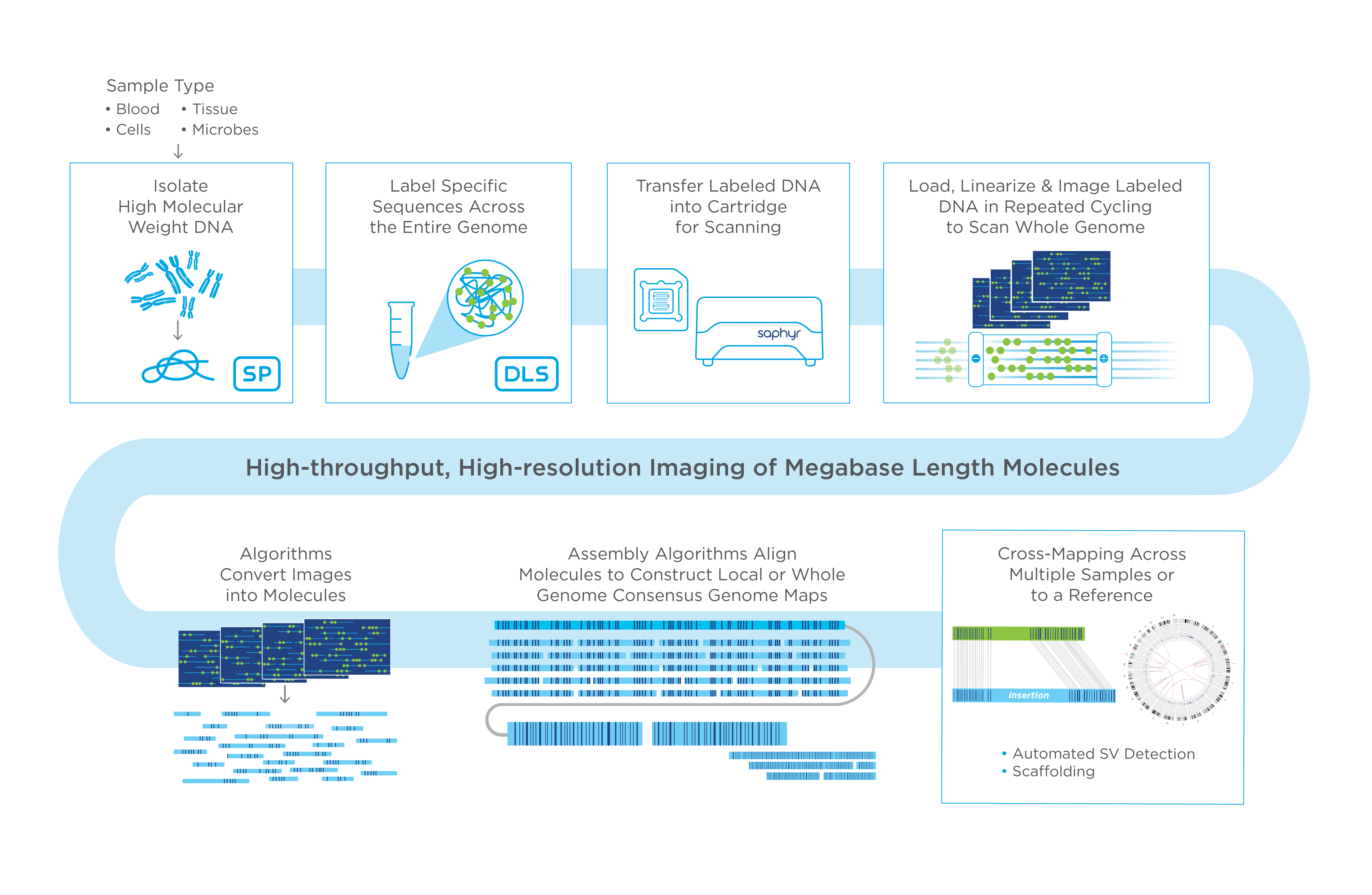
In this step, the linkage information provided by optical maps is integrated with primary assembly sequences, and the overlaps are used to orient and order the contigs, resolve chimeric joins, and estimate the length of gaps between adjacent contigs. One of the advantages of optical maps is that they can easily span genomic regions that are difficult to resolve using DNA sequencing technologies (Savara et al. 2021, Yuan et al. 2020).
Comment: Background on Bionano optical maps
Bionano technology relies on the isolation of kilobase-long DNA fragments, which are labeled at specific sequence motifs with a fluorescent dye, resulting in a unique fluorescent pattern for each genome. DNA molecules are stretched into nanoscale channels and imaged with a high-resolution camera, allowing us to build optical maps that include the physical locations of labels rather than base-level information (Lam et al. 2012, Giani et al. 2020, Savara et al. 2021).
“Estimated reference genome size (in bp) for computing NGx statistics”: 11747076 (previously estimated)
“Type of organism”: Eukaryote (--eukaryote): use of GeneMark-ES for gene finding, Barrnap for ribosomal RNA genes prediction, BUSCO for conserved orthologs finding
In “Genes”:
“Tool for gene prediction”: Don't predict genes
Rename the HTML report as QUAST second report
BuscoTool: toolshed.g2.bx.psu.edu/repos/iuc/busco/busco/5.0.0+galaxy0 with the following parameters:
param-files“Sequences to analyze”: Primary assembly Bionano
“Mode”: Genome assemblies (DNA)
“Use Augustus instead of Metaeuk”: Use Metaeuk
“Auto-detect or select lineage?”: Select lineage
“Lineage”: Saccharomycetes
In “Advanced Options”:
“Which outputs should be generated”: short summary text and summary image
Rename the summary as BUSCO second report
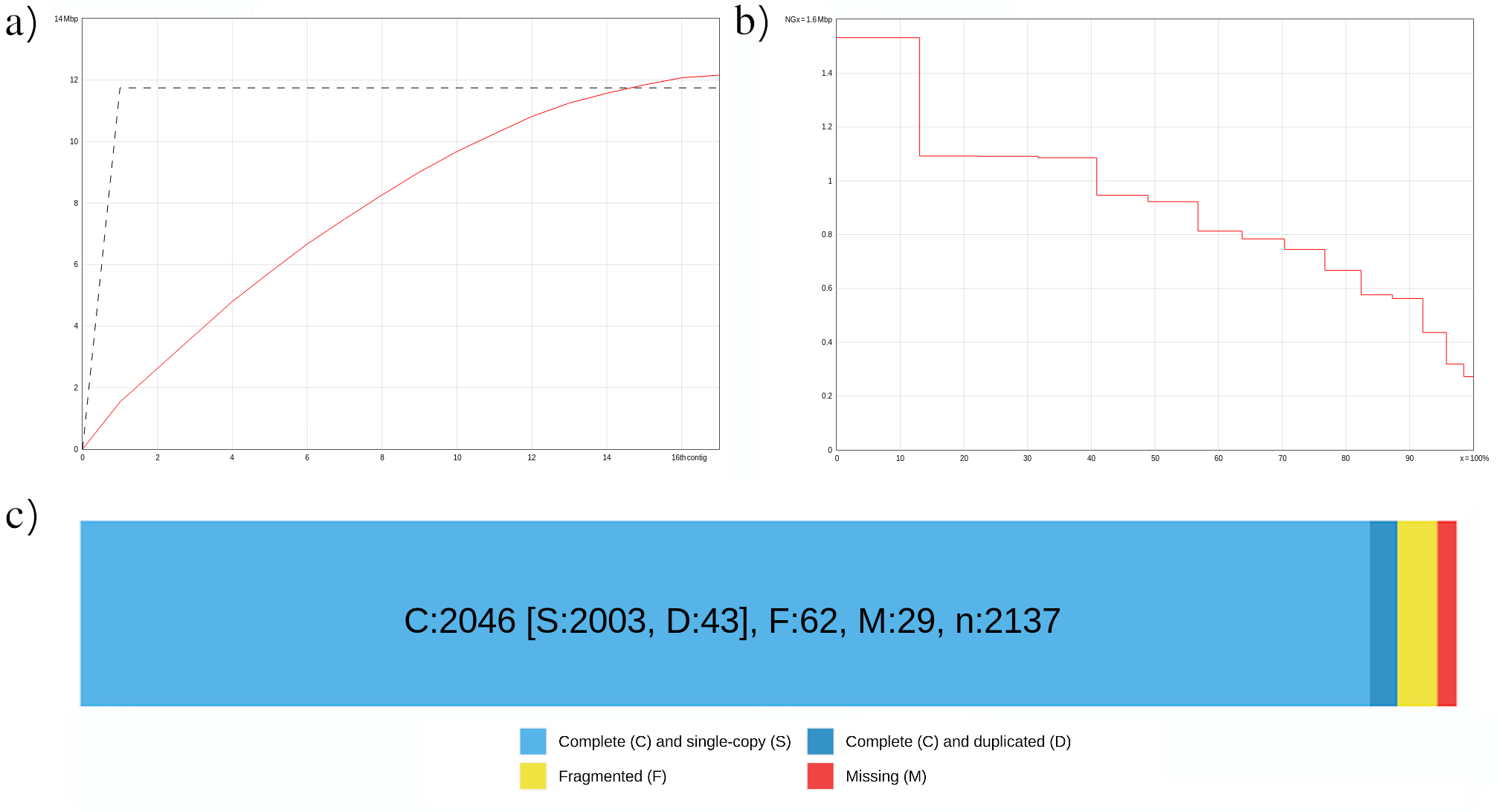
As we can observe in the cumulative plot (fig. 10a), the total length of the assembly (12.160.926 bp) is slightly larger than the expected genome size. With respect to the NG50 statistic (fig. 10b), the value is 922.430 bp, which is significantly higher than the value obtained during the first evaluation stage (813.039 bp).
Figure 10: . Cumulative length plot (a). NGx plot. The y-axis represents the NGx values in Mbp, and the x-axis is the percentage of the genome (b). Assembly evaluation after runnig Bionano. BUSCO genes are defined as "Complete (C) and single copy (S)" when are found once in the single-copy ortholog database, "Complete (C) and duplicated (D)" when single-copy ortholog genes which were found more than once, "Fragmented (F)" when genes are matching just partially to a single-copy ortholog DB, and "Missing (M)" when genes which are expected but were not detected (c).
Finally, the BUSCO’s summary image (fig. 10c) shows that most of the universal single-copy orthologs are present in our assembly.
Question
How many scaffolds are in the primary assembly after the hybrid scaffolding?
What is the size of the largest scaffold? Has improved with respect to the previous evaluation?
What is the percertage of completeness on the core set genes in BUSCO? Has increased the completeness?
The number of contigs is 17.
The largest contig is 1.531.728 bp long. This value hasn’t changed.
The percentage of complete BUSCOs is 95.7%. Yes, it has increased, since in the previous evaluation the completeness percentage was 88.7%.
Hi-C is a sequencing-based molecular assay designed to identify regions of frequent physical interaction in the genome by measuring the contact frequency between all pairs of loci, allowing us to provide an insight into the three-dimensional organization of a genome (Dixon et al. 2012, Lieberman-Aiden et al. 2009). In this final stage, we will exploit the fact that the contact frequency between a pair of loci strongly correlates with the one-dimensional distance between them with the objective of linking the Bionano scaffolds to a chromosome scale.
Comment: Background about Hi-C data
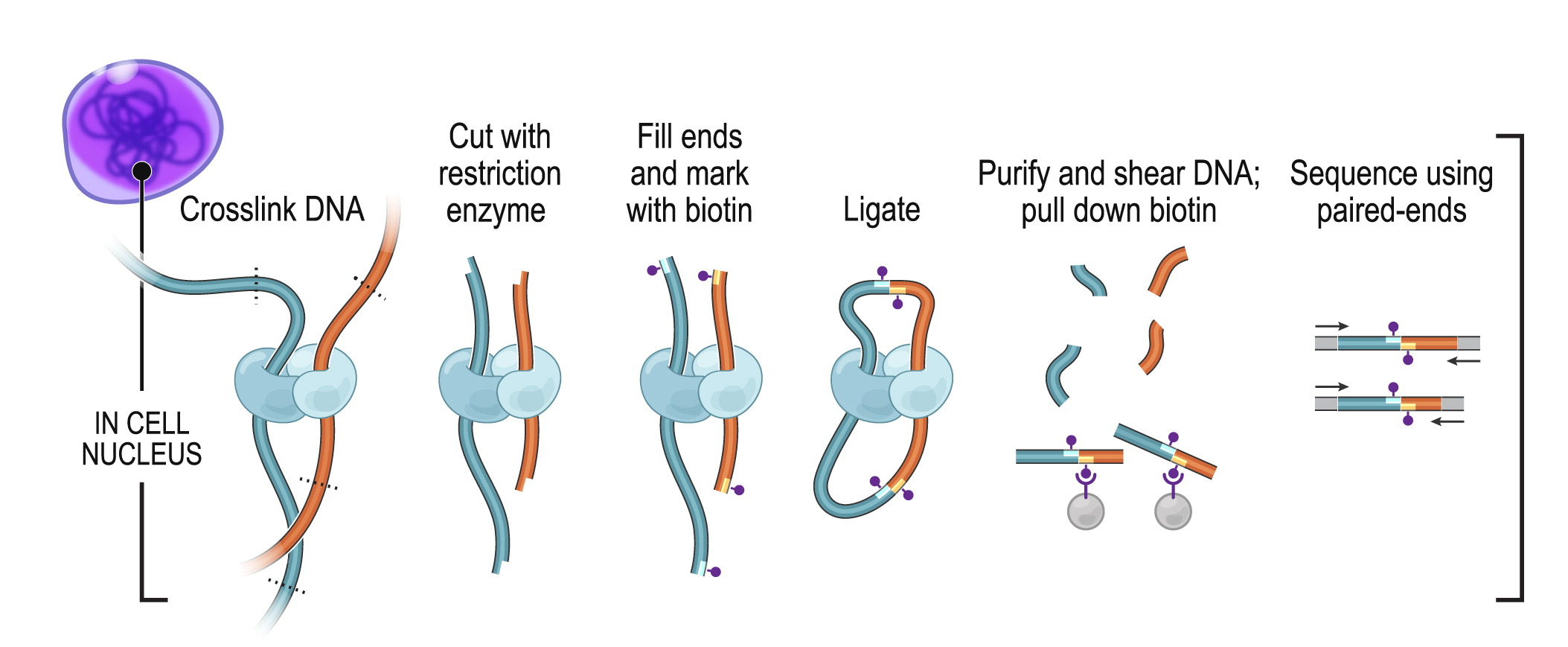
The high-throughput chromosome conformation capture (Hi-C) technology is based on the capture of the chromatin in three-dimensional space. During Hi-C library preparation, DNA is crosslinked in its 3D conformation. Then, the DNA is digested using restriction enzymes, and the digested ends are filled with biotinylated nucleotides (fig. 11). The biotinylated nucleotides enable the specific purification of the ligation junctions, preventing the sequencing of DNA molecules that do not contain such junctions which are thus mostly uninformative (Lajoie et al. 2015).
Figure 11: Hi-C protocol. Adapted from Rao et al. 2014
Next, the blunt ends of the spatially proximal digested end are ligated. Each DNA fragment is then sequenced from each end of this artificial junction, generating read pairs. This provides contact information that can be used to reconstruct the proximity of genomic sequences belonging to the same chromosome (Giani et al. 2020). Hi-C data are in the form of two-dimensional matrices (contact maps) whose entries quantify the intensity of the physical interaction between genome regions.
Pre-processing Hi-C data
Despite Hi-C generating paired-end reads, we need to map each read separately. This is because most aligners assume that the distance between paired-end reads fit a known distribution, but in Hi-C data the insert size of the ligation product can vary between one base pair to hundreds of megabases (Lajoie et al. 2015).
Hands-on: Mapping Hi-C reads
BWA-MEM2Tool: toolshed.g2.bx.psu.edu/repos/iuc/bwa_mem2/bwa_mem2/2.2.1+galaxy0 with the following parameters:
“Will you select a reference genome from your history or use a built-in index?”: Use a genome from history and build index
param-file“Use the following dataset as the reference sequence”: Primary assembly bionano
“Single or Paired-end reads”: Single
param-file“Select fastq dataset”: Hi-C_dataset_F
“Set read groups information?”: Do not set
“Select analysis mode”: 1.Simple Illumina mode
“BAM sorting mode”: Sort by read names (i.e., the QNAME field)
Rename the output as BAM forward
BWA-MEM2Tool: toolshed.g2.bx.psu.edu/repos/iuc/bwa_mem2/bwa_mem2/2.2.1+galaxy0 with the following parameters:
“Will you select a reference genome from your history or use a built-in index?”: Use a genome from history and build index
param-file“Use the following dataset as the reference sequence”: Primary assembly bionano
“Single or Paired-end reads”: Single
param-file“Select fastq dataset”: Hi-C_dataset_R
“Set read groups information?”: Do not set
“Select analysis mode”: 1.Simple Illumina mode
“BAM sorting mode”: Sort by read names (i.e., the QNAME field)
Rename the output as BAM reverse
Filter and mergeTool: toolshed.g2.bx.psu.edu/repos/iuc/bellerophon/bellerophon/1.0+galaxy0 chimeric reads from Arima Genomics with the following parameters:
param-file“First set of reads”: BAM forward
param-file“Second set of reads”: BAM reverse
Rename it as BAM Hi-C reads
Finally, we need to convert the BAM file to BED format and sort it.
Generate initial Hi-C contact map
After mapping the Hi-C reads, the next step is to generate an initial Hi-C contact map, which will allow us to compare the Hi-C contact maps before and after using the Hi-C for scaffolding.
Comment: Biological basis of Hi-C contact maps
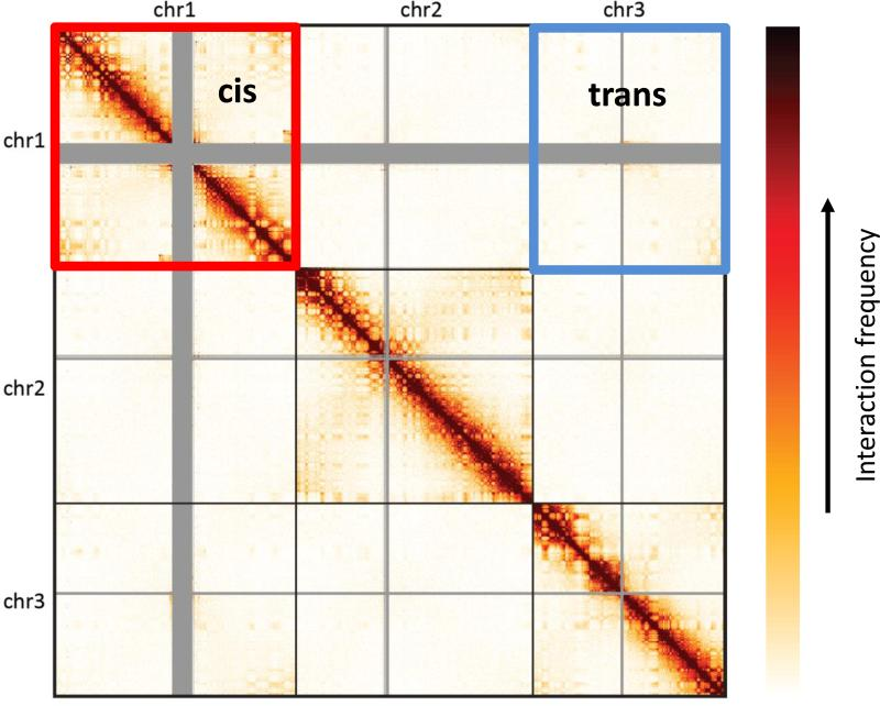
Hi-C contact maps reflect the interaction frequency between genomic loci. In order to understand the Hi-C contact maps, it is necessary to take into account two factors: the higher interaction frequency between loci that reside in the same chromosome (i.e., in cis), and the distance-dependent decay of interaction frequency (Lajoie et al. 2015).
The higher interaction between cis regions can be explained, at least in part, by the territorial organization of chromosomes in interphase (chromosome territories), and in a genome-wide contact map, this pattern appears as blocks of high interaction centered along the diagonal and matching individual chromosomes (fig. 12) (Cremer and Cremer 2010, Lajoie et al. 2015).
Figure 12: An example of a Hi-C map. Genomic regions are arranged along the x and y axes, and contacts are colored on the matrix like a heat map; here darker color indicates greater interaction frequency.
On the other hand, the distance-dependent decay may be due to random movement of the chromosomes, and in the contact map appears as a gradual decrease of the interaction frequency the farther away from the diagonal it moves (Lajoie et al. 2015).
Hands-on: Generate a contact map with PretextMap and Pretext Snapshot
PretextMapTool: toolshed.g2.bx.psu.edu/repos/iuc/pretext_map/pretext_map/0.1.6+galaxy0 with the following parameters:
param-file“Input dataset in SAM or BAM format”: BAM Hi-C reads
“Sort by”: Don't sort
Rename the output as PretextMap output
Pretext SnapshotTool: toolshed.g2.bx.psu.edu/repos/iuc/pretext_snapshot/pretext_snapshot/0.0.3+galaxy0 with the following parameters:
Let’s have a look at the Hi-C contact maps generated by Pretext Snapshot.
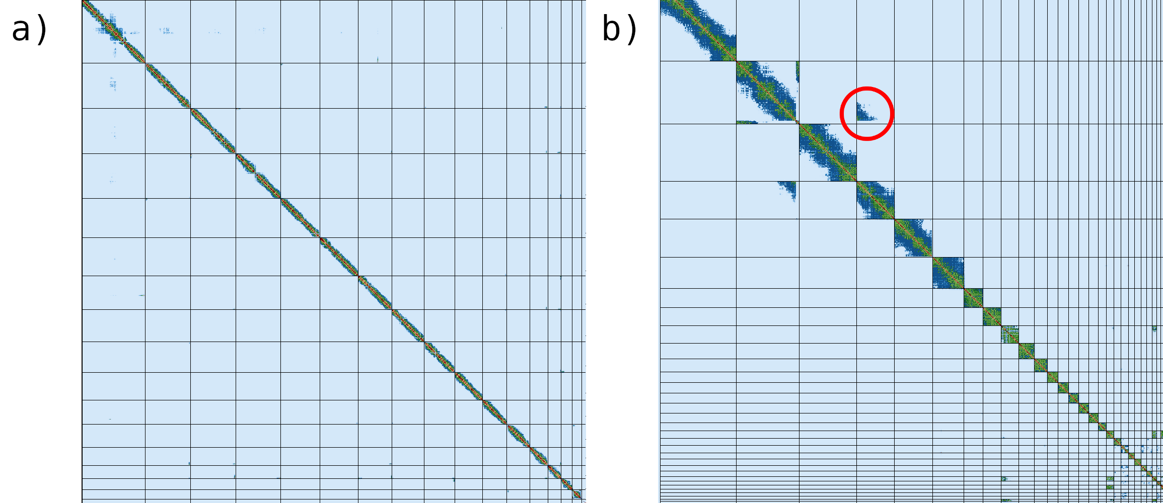
Figure 13: Hi-C map generated by Pretext. Primary assembly full contact map generated in this training (a) Hi-C map representative of a typical missasembly (b).
In the contact generated from the Bionano-scaffolded assembly can be identified 17 scaffolds, representing each of the haploid chromosomes of our genome (fig. 13.a). The fact that all the contact signals are found around the diagonal suggest that the contigs were scaffolded in the right order. However, during the assembly of complex genomes, it is common to find in the contact maps indicators of errors during the scaffolding process, as shown in the figure 13b. In that case, a contig belonging to the second chromosome has been misplaced as part of the fourth chromosome. We can also note that the final portion of the second chromosome should be placed at the beginning, as the off-diagonal contact signal suggests.
Once we have evaluated the quality of the scaffolded genome assembly, the next step consists in integrating the information contained in the HiC reads into our assembly, so that any errors identified can be resolved. For this purpose we will use SALSA2 (Ghurye et al. 2019).
SALSA2 scaffolding
SALSA2 is an open source software that makes use of Hi-C to linearly orient and order assembled contigs along entire chromosomes (Ghurye et al. 2019). One of the advantages of SALSA2 with respect to most existing Hi-C scaffolding tools is that it doesn’t require the estimated number of chromosomes.
Comment: SALSA2 algorithm overview
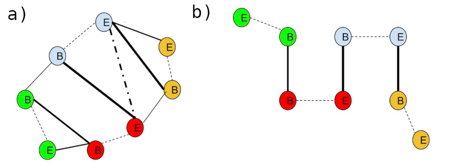
Initially SALSA2 uses the physical coverage of Hi-C pairs to identify suspicious regions and break the sequence at the likely point of mis-assembly. Then, a hybrid scaffold graph is constructed using edges from the Hi-C reads, scoring the edges according to a best buddy scheme (fig. 14a).
Figure 14: Overview of the SALSA2 algorithm. Solid edges indicate the linkages between different contigs and dotted edges indicate the links between the ends of the same contig. B and E denote the start and end of contigs, respectively. Adapted from Ghurye et al. 2019.
From this graph scaffolds are iteratively constructed using a greedy weighted maximum matching. After each iteration, a mis-join detection step is performed to check if any of the joins made during this round are incorrect. Incorrect joins are broken and the edges blacklisted during subsequent iterations. This process continues until the majority of joins made in the prior iteration are incorrect. This provides a natural stopping condition, when accurate Hi-C links have been exhausted (Ghurye et al. 2019).
Before launching SALSA2, we need to carry out some modifications on our datasets.
Hands-on: BAM to BED conversion
bedtools BAM to BEDTool: toolshed.g2.bx.psu.edu/repos/iuc/bedtools/bedtools_bamtobed/2.30.0+galaxy1 with the following parameters:
param-file“Convert the following BAM file to BED”: BAM Hi-C reads
“What type of BED output would you like”: Create a full, 12-column "blocked" BED file
Rename the output as BED unsorted
SortTool: sort1 with the following parameters:
param-file“Sort Dataset”: BED unsorted
“on column”: Column: 4
“with flavor”: Alphabetical sort
“everything in”: Ascending order
Rename the output as BED sorted
ReplaceTool: toolshed.g2.bx.psu.edu/repos/bgruening/text_processing/tp_find_and_replace/1.1.3 with the following parameters:
param-file“File to process”: Primary assembly bionano
“Find pattern”: :
“Replace all occurrences of the pattern”: Yes
“Find and Replace text in”: entire line
Rename the output as Primary assembly bionano edited
Now we can launch SALSA2 in order to generate the hybrid scaffolding based on the Hi-C data.
Hands-on: Salsa scaffolding
SALSATool: toolshed.g2.bx.psu.edu/repos/iuc/salsa/salsa/2.3+galaxy0 with the following parameters:
Rename the output as SALSA2 scaffold FASTA and SALSA2 scaffold AGP
Evaluate the final genome assembly with Pretext
Finally, we should repeat the procedure described previously for generating the contact maps, but in that case, we will use the scaffold generated by SALSA2.
Hands-on: Mappingreads against the scaffold
BWA-MEM2Tool: toolshed.g2.bx.psu.edu/repos/iuc/bwa_mem2/bwa_mem2/2.2.1+galaxy0 with the following parameters:
“Will you select a reference genome from your history or use a built-in index?”: Use a genome from history and build index
param-file“Use the following dataset as the reference sequence”: SALSA2 scaffold FASTA
“Single or Paired-end reads”: Single
param-file“Select fastq dataset”: Hi-C_dataset_F
“Set read groups information?”: Do not set
“Select analysis mode”: 1.Simple Illumina mode
“BAM sorting mode”: Sort by read names (i.e., the QNAME field)
Rename the output as BAM forward SALSA2
BWA-MEM2Tool: toolshed.g2.bx.psu.edu/repos/iuc/bwa_mem2/bwa_mem2/2.2.1+galaxy0 with the following parameters:
“Will you select a reference genome from your history or use a built-in index?”: Use a genome from history and build index
param-file“Use the following dataset as the reference sequence”: SALSA2 scaffold FASTA
“Single or Paired-end reads”: Single
param-file“Select fastq dataset”: Hi-C_dataset_R
“Set read groups information?”: Do not set
“Select analysis mode”: 1.Simple Illumina mode
“BAM sorting mode”: Sort by read names (i.e., the QNAME field)
Rename the output as BAM reverse SALSA2
Filter and mergeTool: toolshed.g2.bx.psu.edu/repos/iuc/bellerophon/bellerophon/1.0+galaxy0 chimeric reads from Arima Genomics with the following parameters:
param-file“First set of reads”: BAM forward SALSA2
param-file“Second set of reads”: BAM reverse SALSA2
Rename the output as BAM Hi-C reads SALSA2
PretextMapTool: toolshed.g2.bx.psu.edu/repos/iuc/pretext_map/pretext_map/0.1.6+galaxy0 with the following parameters:
param-file“Input dataset in SAM or BAM format”: BAM Hi-C reads SALSA2
“Sort by”: Don't sort
Rename the output as PretextMap output SALSA2
Pretext SnapshotTool: toolshed.g2.bx.psu.edu/repos/iuc/pretext_snapshot/pretext_snapshot/0.0.3+galaxy0 with the following parameters:
In order to evaluate the Hi-C hybrid scaffolding, we are going to compare the contact maps before and after running SALSA2 (fig. 15).
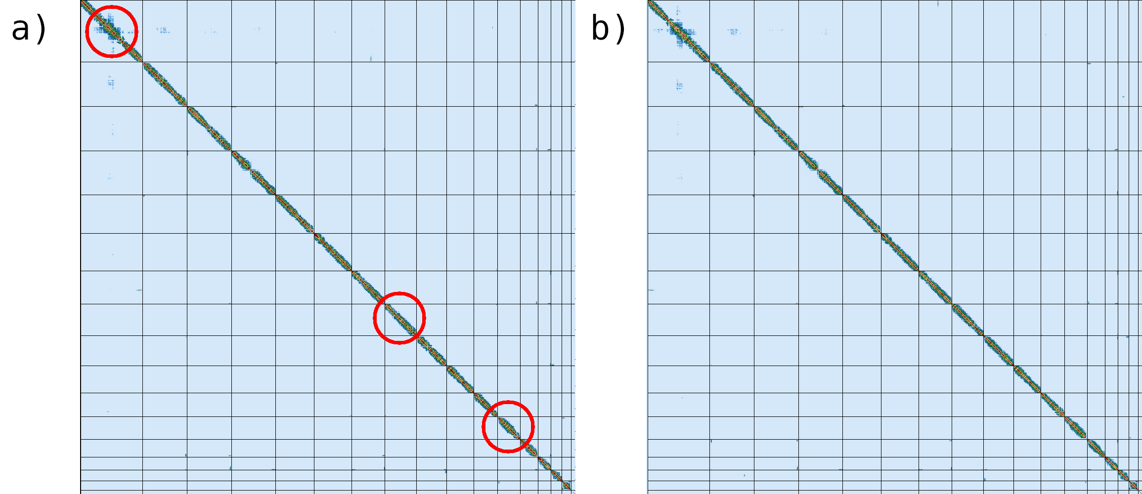
Figure 15: Hi-C map generated by Pretext after the hybrid scaffolding based on Hi-C data. The red circles indicate the differences between the contact map generated after (a) and before (b) Hi-C hybrid scaffolding.
Among the most notable differences that can be identified between the contact maps, it can be highlighted the regions marked with red circles, where inversion can be identified.
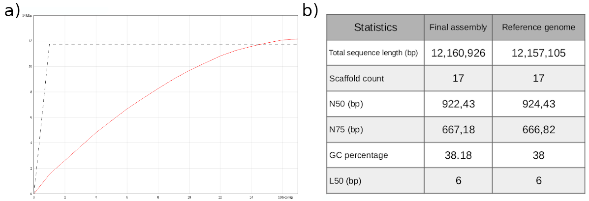
Figure 16: Comparison between the final assembly generating in this training and the reference genome. Contiguity plot using the reference genome size (a). Assemby statistics (b).
With respect to the total sequence length, we can conclude that the size of our genome assembly is almost identical to the reference genome (fig.16a,b). Regarding the number of scaffolds, the obtained value is similar to the reference assembly, which consist in 16 chromosomes plus the mitochondrial DNA, which consists of 85,779 bp. The remaining statistics exhibit very similar values (fig. 16b).
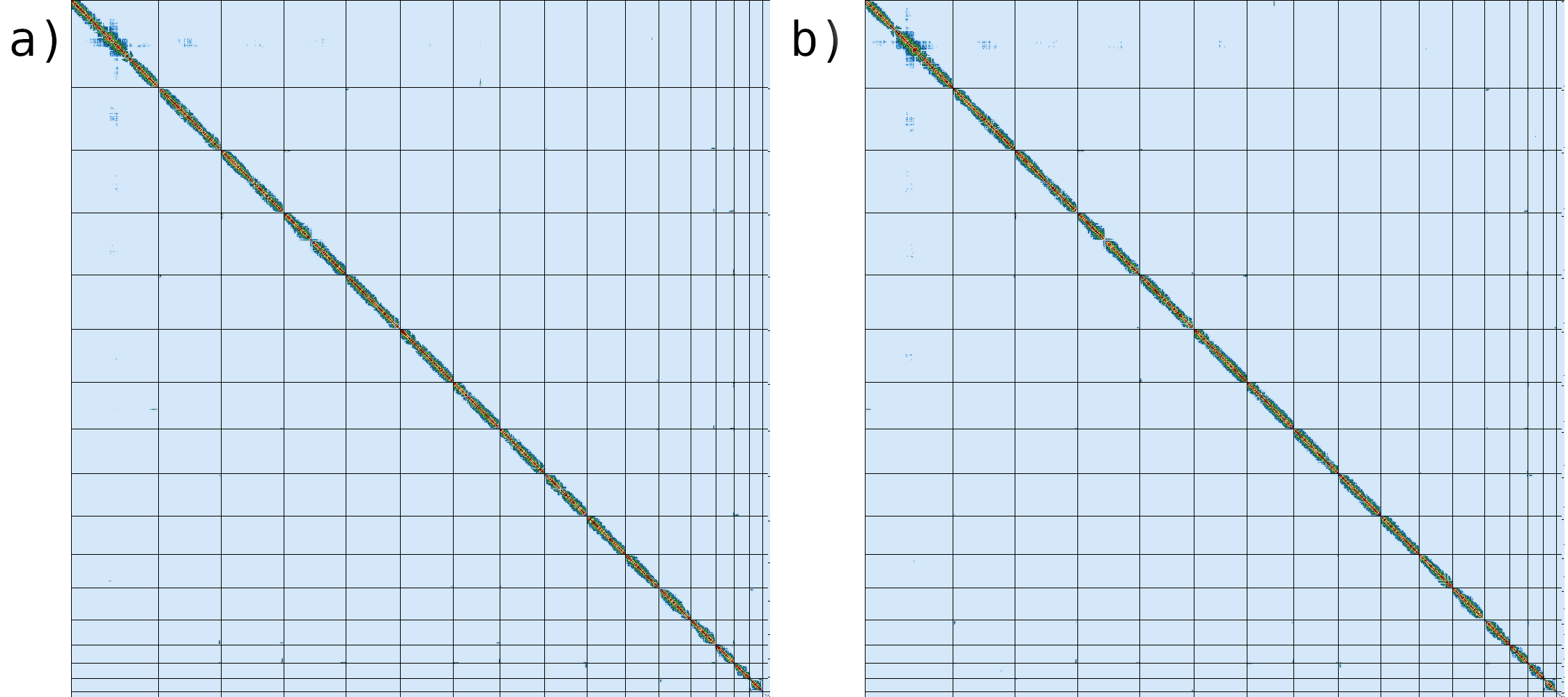
Figure 17: Comparison between contact maps generated by using the final assembly (a) and the reference genome (b).
If we compare the contact map of our assembled genome (fig. 17a) with the reference assembly (fig. 17b), we can see that the two are essentially identical. This means that we have achieved an almost perfect assembly at the chromosome level.
Key points
The VGP pipeline allows to generate error-free, near gapless reference-quality genome assemblies
The assembly can be divided in four main stages: genome profile analysis, HiFi long read phased assembly with hifiasm, Bionano hybrid scaffolding and Hi-C hybrid scaffolding
Marcotte, E. M., M. Pellegrini, T. O. Yeates, and D. Eisenberg, 1999 A census of protein repeats. Journal of Molecular Biology 293: 151–160. 10.1006/jmbi.1999.3136
Small, K. S., M. Brudno, M. M. Hill, and A. Sidow, 2007 A haplome alignment and reference sequence of the highly polymorphic Ciona savignyi genome. Genome Biology 8: R41. 10.1186/gb-2007-8-3-r41
Lieberman-Aiden, E., N. L. van Berkum, L. Williams, M. Imakaev, T. Ragoczy et al., 2009 Comprehensive Mapping of Long-Range Interactions Reveals Folding Principles of the Human Genome. Science 326: 289–293. 10.1126/science.1181369
Cremer, T., and M. Cremer, 2010 Chromosome Territories. Cold Spring Harbor Perspectives in Biology 2: a003889–a003889. 10.1101/cshperspect.a003889
Dixon, J. R., S. Selvaraj, F. Yue, A. Kim, Y. Li et al., 2012 Topological domains in mammalian genomes identified by analysis of chromatin interactions. Nature 485: 376–380. 10.1038/nature11082
Frenkel, S., V. Kirzhner, and A. Korol, 2012 Organizational Heterogeneity of Vertebrate Genomes (V. Laudet, Ed.). PLoS ONE 7: e32076. 10.1371/journal.pone.0032076
Lam, E. T., A. Hastie, C. Lin, D. Ehrlich, S. K. Das et al., 2012 Genome mapping on nanochannel arrays for structural variation analysis and sequence assembly. Nature Biotechnology 30: 771–776. 10.1038/nbt.2303
Chalopin, D., M. Naville, F. Plard, D. Galiana, and J.-N. Volff, 2015 Comparative Analysis of Transposable Elements Highlights Mobilome Diversity and Evolution in Vertebrates. Genome Biology and Evolution 7: 567–580. 10.1093/gbe/evv005
Lajoie, B. R., J. Dekker, and N. Kaplan, 2015 The Hitchhiker’s guide to Hi-C analysis: Practical guidelines. Methods 72: 65–75. 10.1016/j.ymeth.2014.10.031
Simão, F. A., R. M. Waterhouse, P. Ioannidis, E. V. Kriventseva, and E. M. Zdobnov, 2015 BUSCO: assessing genome assembly and annotation completeness with single-copy orthologs. Bioinformatics 31: 3210–3212. 10.1093/bioinformatics/btv351
Sotero-Caio, C. G., R. N. Platt, A. Suh, and D. A. Ray, 2017 Evolution and Diversity of Transposable Elements in Vertebrate Genomes. Genome Biology and Evolution 9: 161–177. 10.1093/gbe/evw264
Angel, V. D. D., E. Hjerde, L. Sterck, S. Capella-Gutierrez, C. Notredame et al., 2018 Ten steps to get started in Genome Assembly and Annotation. F1000Research 7: 148. 10.12688/f1000research.13598.1
Roach, M. J., S. A. Schmidt, and A. R. Borneman, 2018 Purge Haplotigs: allelic contig reassignment for third-gen diploid genome assemblies. BMC Bioinformatics 19: 10.1186/s12859-018-2485-7
Ghurye, J., A. Rhie, B. P. Walenz, A. Schmitt, S. Selvaraj et al., 2019 Integrating Hi-C links with assembly graphs for chromosome-scale assembly (I. Ioshikhes, Ed.). PLOS Computational Biology 15: e1007273. 10.1371/journal.pcbi.1007273
Guan, D., S. A. McCarthy, J. Wood, K. Howe, Y. Wang et al., 2019 Identifying and removing haplotypic duplication in primary genome assemblies. 10.1101/729962
Tørresen, O. K., B. Star, P. Mier, M. A. Andrade-Navarro, A. Bateman et al., 2019 Tandem repeats lead to sequence assembly errors and impose multi-level challenges for genome and protein databases. Nucleic Acids Research 47: 10994–11006. 10.1093/nar/gkz841
Giani, A. M., G. R. Gallo, L. Gianfranceschi, and G. Formenti, 2020 Long walk to genomics: History and current approaches to genome sequencing and assembly. Computational and Structural Biotechnology Journal 18: 9–19. 10.1016/j.csbj.2019.11.002
Hon, T., K. Mars, G. Young, Y.-C. Tsai, J. W. Karalius et al., 2020 Highly accurate long-read HiFi sequencing data for five complex genomes. Scientific Data 7: 10.1038/s41597-020-00743-4
Ranallo-Benavidez, T. R., K. S. Jaron, and M. C. Schatz, 2020 GenomeScope 2.0 and Smudgeplot for reference-free profiling of polyploid genomes. Nature Communications 11: 10.1038/s41467-020-14998-3
Rhie, A., B. P. Walenz, S. Koren, and A. M. Phillippy, 2020 Merqury: reference-free quality, completeness, and phasing assessment for genome assemblies. Genome Biology 21: 10.1186/s13059-020-02134-9
Wang, H., B. Liu, Y. Zhang, F. Jiang, Y. Ren et al., 2020 Estimation of genome size using k-mer frequencies from corrected long reads. arXiv preprint arXiv:2003.11817. https://arxiv.org/abs/2003.11817
Yuan, Y., C. Y.-L. Chung, and T.-F. Chan, 2020 Advances in optical mapping for genomic research. Computational and Structural Biotechnology Journal 18: 2051–2062. 10.1016/j.csbj.2020.07.018
Zhang, X., R. Wu, Y. Wang, J. Yu, and H. Tang, 2020 Unzipping haplotypes in diploid and polyploid genomes. Computational and Structural Biotechnology Journal 18: 66–72. 10.1016/j.csbj.2019.11.011
Cheng, H., G. T. Concepcion, X. Feng, H. Zhang, and H. Li, 2021 Haplotype-resolved de novo assembly using phased assembly graphs with hifiasm. Nature Methods 18: 170–175. 10.1038/s41592-020-01056-5
Dida, F., and G. Yi, 2021 Empirical evaluation of methods for de novo genome assembly. PeerJ Computer Science 7: e636. 10.7717/peerj-cs.636
Rhie, A., S. A. McCarthy, O. Fedrigo, J. Damas, G. Formenti et al., 2021 Towards complete and error-free genome assemblies of all vertebrate species. Nature 592: 737–746. 10.1038/s41586-021-03451-0
Savara, J., T. Novosád, P. Gajdoš, and E. Kriegová, 2021 Comparison of structural variants detected by optical mapping with long-read next-generation sequencing (C. Kendziorski, Ed.). Bioinformatics 37: 3398–3404. 10.1093/bioinformatics/btab359
Feedback
Did you use this material as an instructor? Feel free to give us feedback on how it went.
Did you use this material as a learner or student? Click the form below to leave feedback.
Batut et al., 2018 Community-Driven Data Analysis Training for Biology Cell Systems 10.1016/j.cels.2018.05.012
@misc{assembly-vgp_genome_assembly,
author = "Delphine Lariviere and Alex Ostrovsky and Cristóbal Gallardo and Anna Syme and Linelle Abueg and Brandon Pickett and Giulio Formenti and Marcella Sozzoni",
title = "VGP assembly pipeline (Galaxy Training Materials)",
year = "",
month = "",
day = ""
url = "\url{https://training.galaxyproject.org/training-material/topics/assembly/tutorials/vgp_genome_assembly/tutorial.html}",
note = "[Online; accessed TODAY]"
}
@article{Batut_2018,
    doi = {10.1016/j.cels.2018.05.012},
    url = {https://doi.org/10.1016%2Fj.cels.2018.05.012},
    year = 2018,
    month = {jun},
    publisher = {Elsevier {BV}},
    volume = {6},
    number = {6},
    pages = {752--758.e1},
    author = {B{\'{e}}r{\'{e}}nice Batut and Saskia Hiltemann and Andrea Bagnacani and Dannon Baker and Vivek Bhardwaj and Clemens Blank and Anthony Bretaudeau and Loraine Brillet-Gu{\'{e}}guen and Martin {\v{C}}ech and John Chilton and Dave Clements and Olivia Doppelt-Azeroual and Anika Erxleben and Mallory Ann Freeberg and Simon Gladman and Youri Hoogstrate and Hans-Rudolf Hotz and Torsten Houwaart and Pratik Jagtap and Delphine Larivi{\`{e}}re and Gildas Le Corguill{\'{e}} and Thomas Manke and Fabien Mareuil and Fidel Ram{\'{\i}}rez and Devon Ryan and Florian Christoph Sigloch and Nicola Soranzo and Joachim Wolff and Pavankumar Videm and Markus Wolfien and Aisanjiang Wubuli and Dilmurat Yusuf and James Taylor and Rolf Backofen and Anton Nekrutenko and Björn Grüning},
    title = {Community-Driven Data Analysis Training for Biology},
    journal = {Cell Systems}
}
Congratulations on successfully completing this tutorial!
 Delphine Lariviere
 Alex Ostrovsky
 Cristóbal Gallardo
 Anna Syme
 Linelle Abueg
 Brandon Pickett
 Giulio Formenti
 Marcella Sozzoni
 Questions: